NLS方程式のホモクリニック解と数値的周期性(計算流体力学に関わる数理的諸問題)

(1)

NLS

方程式のホモクリニック解と数値的周期性

東大理梅木誠

Generalized homoclinic solutions and numerical periodicity of the NLS equation Makoto Umeki

Department of Physics, University of Tokyo Abstract

A generalization is given of the Ablowitz &Herbst’s exact

solu-tions ofthe nonlinear Schrdinger (NLS) equation, which are

tempo-rally homoclinic and periodic in space. It is found that, in numerical

simulations ofthe integrable difference scheme of the NLS equation,

periodic and quasi-periodic motions are generated instead of $\mathrm{h}\mathrm{o}\mathrm{m}(\succ$

clinic orbits. The periods are proportional to $-\ln\epsilon/\Omega_{i}$, where $\epsilon$ is

the magnitudeof numerical errors and $\Omega_{i}$ is the growth rate of the

unstable modes.

Homoclinicity in dynamical systems plays acrucial role in understanding

a mechanismof creationof chaos. Inlow-dimensional systems, it is knownas

the Melnikov’s theorem that a perturbation often destroys the unperturbed

homoclinic orbits in integrable systems and create the Smale’s horseshoe

mapping inthevicinity of them. Inthissense,homoclinicitymaybe regarded

as the

_fouffi

_{route to chaos, in addition to period-doubling, quasi-periodicity}

and intermittency. In contrast withlow-dimensional systems,thehomoclinic

structures in higher or infinite dimensions have been studied very recently

[1, 3, 4, 6] and the study should be applied to physical phenomena including

parametrically forced water waves [7].

On the other hand, the nonlinear Schr\"odinger equation, which is one of

themost-understood integrable equationsby soliton theory, is still attractive

for study ifweconsideritsperiodicboundaryproblem. Inaremarkablepaper

[1] Ablowitz and Herbst first showed that the focusingnonlinearSchr\"odinger

equation

$iu_{t}+u_{xx}+2\sigma|u|^{2}u=0$, (1)

with $\sigma=1$ possesses analytically expressed exact solutions which are

homo-clinic to the periodic solution $u=a$$\exp 2ia^{2}t$. The $N$-homoclinic solution

was derived through the transform $xarrow ix,$$tarrow-t$ of 2N-dark-hole

(2)

with $\sigma=-1$ ) with the evenness condition $u(x, t)=u(-x, t)$, which can

be derived directly by Hirota’s bilinear method. However, we show that the

evenness condition is just sufficient but not necessary.

The $M-\mathrm{d}\mathrm{a}\Gamma \mathrm{k}$-hole soliton solutionof thedefocusing NLSequation is given

by

$u(x,t)=a\exp(-2ia^{2}t)g(x,t)/f(x, t)$, (2) where

$f(x,t)= \sum_{=\tilde{\mu}0,1}\exp[\sum_{j>k}^{M}\alpha_{jk\mu_{j}}\mu_{k}+\sum_{j}M=1\mu_{j}\eta_{j}]$ , (3)

$g(x, t)= \sum_{\overline{\mu}=0,1}\exp[\sum_{j>k}^{M}\alpha jk\mu j\mu k+\sum_{1j=}\mu j(\eta_{j}+2iM\phi_{j})]$ , (4)

and

$\exp(\alpha_{jk})=[\frac{\sin(\phi_{j}-\phi_{k})/2}{\sin(\phi_{j}+\phi_{k})/2}]^{2}$ (5)

$\eta_{j}=p_{j}(x-X_{j})-\Omega_{j}t+\gamma_{j}$ (6)

$p_{j}=2a\sin\phi_{j}$ (7)

$\Omega_{j}=\pm p_{j}\sqrt{4a^{2}-p_{j}^{2}}$, (8) $\phi_{j},$ $\gamma_{j}$ and $x_{j}$ are real constants, $\sum_{\overline{\mu}=0,1}$ is the summation over all possible

combination of$\mu_{j}=0$ and 1 for $j=1,$$\cdots,$$M$ and $\sum_{j>k}^{M}$ denotes the

sum-mation over all possible pairs chosen from $M$ elements. Here the definition

of the phase $\gamma_{j}$ is different ffom that in [1] since we introduced $x_{j}$. In order

to obtaingeneral homoclinic solutions, we put

$x=iX,$ $t=-T$ and $x_{j}=iX_{j}$

.

(9)

We denote, under the above transform, the relation between the solutions $u$

and $U$ ofthe defocusing and focusingNLS equations, respectively, as

$u(x, t;x_{j})=U(x, T;x_{j})$. (10)

Theremaining condition that we should impose is the real-valuedness of

$f(x, t)$

.

This cannot be not satisfied if $M$ is odd, but if$M$ is even, it can be

satisfied by letting $p_{2j-1}=-p2j,$$\gamma 2j-1=\gamma_{2j},$ $\Omega_{2j-1}=\Omega_{2j},$$\phi_{2j-}1=\phi_{2j}+\pi$

(3)

not only periodic solutions in space but also quasi-periodic solutions if$p_{j}$ are

incommensurate.

The solutionfor $N=1$ is given explicitlyby

$U(X,T)=a \mathrm{e}\frac{1+2\cos\varphi \mathrm{e}^{\theta+i}\emptyset+A_{12}22\mathrm{e}\theta+4i\emptyset}{1+2\cos\varphi \mathrm{e}^{\theta}+A12\mathrm{e}2\theta}2ia^{2}T$, (11)

where $\theta=\Omega T+\gamma,$ $\varphi=p(X-X_{1}),$ $p=2a\sin\phi$ and $A_{12}=\cos^{-2}\phi_{\mathrm{J}}$ The

asymptotic behaviors of$U(X, T)$ as $Tarrow\pm\infty$ are respectively given by

$U_{-}=a\mathrm{e}^{2iaT}2[1+4i\sin\phi \mathrm{e}^{\theta}\cos\varphi]+i\emptyset$ , (12)

$U_{+}=a\mathrm{e}^{2ia^{2}}[T+4i\phi 1-4iA^{-1}12\sin\phi \mathrm{e}-\theta-i\emptyset\cos\varphi]$ . (13)

Thereisnoessentialdifference between [1] and thepresentsolutionfor$N=\dot{1}$,

since the solution is invariant under the translation. If $N=2$, however, we

obtain afamily ofnew solutions

$U(X, T;X_{j})=a\exp(2ia2T)G(x, T)/F(X, T)$ ₍₁₄₎

where

$G(X, T)$ $=$ $1+2\mathrm{e}^{\theta_{1+}}2i\phi 1\cos\varphi_{1}+A_{12}\mathrm{e}^{2\theta_{1}4}+i\phi 1+2\mathrm{e}^{\theta 2i}\mathrm{c}\mathrm{o}3+\emptyset 3\mathrm{s}\varphi_{3}$ $+A_{\mathrm{s}}4\mathrm{e}+2\theta_{3+}4i\phi s2\mathrm{e}2\theta_{1+3+}\theta i(\emptyset 1+\phi 3)\{A_{13}\cos(\varphi_{1}+\varphi_{3})$

$+A_{2\mathrm{s}^{\mathrm{c}}}\mathrm{o}\mathrm{s}(\varphi 1-\varphi_{3})\}+2A_{13}A2\mathrm{s}A\mathrm{s}4\mathrm{e}^{\theta 2\theta}1+3+i(2\emptyset 1+4\emptyset 3)\mathrm{c}:0.\mathrm{s}\varphi_{1}$

$+2A_{12}A13A23\mathrm{e}2\theta_{1}+\theta 3+i(4\phi_{1+}2\phi \mathrm{s})\cos\varphi_{\mathrm{s}}$

$+A_{12}A_{1}^{2}3A^{2}23A34\mathrm{e}^{2()+4}\theta_{1}+\theta_{3}i(\phi 1+\phi_{3})$ (15)

and

$F(X, T)=G(X, T)$ with $\phi_{i}=0$ for all $i$, (16)

where$\theta_{i}=\Omega_{i}T+\gamma_{i}$and _{$\varphi_{i}=p_{i}$}(X-Xi). We seethat there exists necessarily

aconjugate counterpart ofeverycomplexterm in (4) under thetransform (9)

for arbitrary $N$, which implies that the real valuedness of$f$ is satisfied. Note

that thereis apossibility of the applicationof this solution to the motion of

a knotted closed filament.

Next, we show how these homoclinic solutions

are

affected by numerical

(4)

precise as possible and examine the effect of errors, we perform a following

numerical experiment.

1) We adapt the Ablowitz-Ladik system [2]

$iu_{nt}+(u_{n+1^{-}}2u_{n}+u_{n-1})/h^{2}+|u_{n}|^{2}(u_{n+1}+u_{n-1})=0$, (17)

whichis the integrablefinite-differenceschemeanddoes not showanychaotic

motions. The number ofspatial discretization $N_{p}$ is taken as 64.

2) We use three numerical codes written in single, double and quadruple

precisions, which have about 7, 16 and 33 effective decimal digits offloating

point numbers. The truncation error is reduced to the level ofthe round-off

error. For this purpose, we choose as the scheme of time integration the

$\mathrm{f}_{\mathrm{o}\mathrm{u}\mathrm{r}\mathrm{t}}.\mathrm{h}$-order Runge-Kutta method in the former two

codes, and the

sixth-order eight-stage method by $\mathrm{H}\mathrm{u}\mathrm{t}\mathrm{a}[5]$ in the quadruple case. The temporal

steplength$\Delta t$ is takenas _{$\Delta t=10^{-2},10^{-}3$} and $10^{-4}$ so that thelocal

trunca-tionerroris roughly estimated as $10^{-8},10^{-}15$ and $10^{-28}$, which are on a level

of the round-off

errors.

Then, we denote the total size of the local numerical

error by $\epsilon_{n}$

3) The initial conditionsaregiven according to the asymptotic form$Tarrow-\infty$

of the solution, (12) for $N=1$. They are expressed by the

sum

of the fixed

point $a$$\exp(2ia^{2}\tau)$ plus a small disturbance which denotes unstable modes.

The magnitude of the disturbance is $\epsilon_{n}$. This may be considered as one of

the best implementations ofhomoclinic orbits in a numericalsense.

First, a 1-homoclinic solution is examined. We put $L=2\sqrt{2}\pi$ and the

initial condition is

$U(X, T=0)=0.5[1-\epsilon(1+i)\cos(pX)]$ ₍₁₈₎

with $p=2\pi/L$ and $\epsilon=\epsilon_{i}=\epsilon_{n}$

.

The $\mathrm{s}\mathrm{p}\mathrm{a}\mathrm{t}\mathrm{i}\mathrm{c}\succ \mathrm{t}\mathrm{e}\mathrm{m}\mathrm{p}\mathrm{o}\mathrm{r}\mathrm{a}\mathrm{l}$ behavior of _$|U|$ in

Figure 1 shows not homoclinic but periodic motion in time. We observe

the sequence of appearance of bumps, whose positions are fixed or changed

alternatively. It should be noted that the periodsof three

cases

are different.

The lefi side of Figure 2 shows the temporal evolution of the amplitude

$A=\sqrt{|\tilde{U}_{1}|^{2}+|\tilde{U}-1|}$where the Fourier coefficients $\tilde{U}_{j}$ is defined by

$\tilde{U}_{j}=\frac{1}{N_{p}}\sum_{l=1}U(x_{\iota})N_{\mathrm{p}}\mathrm{e}-ikjX_{l}$,

(5)

Theright sideof Figure 2shows the temporal plots of$({\rm Re}(V), {\rm Im}(V))$ at $X=$

$0$, where a new variable $V=U\exp(-2ia^{2}\tau)$ is introduced. This periodic

motion and its period can be explained as follows.

The initial condition is expressedas

$V=0.5+\epsilon_{i}\exp(i\varphi i)\cos(pX)$

.

(20) Comparing (12) with (18), we may estimate$\epsilon_{i}\approx\exp(\Omega T_{i}+\gamma)$ and

$T_{i}=(\ln\epsilon_{i}-\gamma)/\Omega$ (21)

Similarly, we can estimate the final time $T_{f}$ of the single bump. The final

statemay be approximated as

$V=\exp(4i\phi)[0.5+\epsilon_{f}\exp(i\varphi_{f})\cos(px)]$. (22)

Letting $\epsilon_{f}\approx\exp[-(\Omega T_{f}+\gamma)]$, we have

$T_{f}=-(\ln\epsilon_{f}+\gamma)/\Omega$ (23)

Then, the lifetime ofthe numerical homoclinic solution is

$T_{f}-T_{C}=-(\ln\epsilon i+\ln\epsilon_{n})/\Omega$ (24)

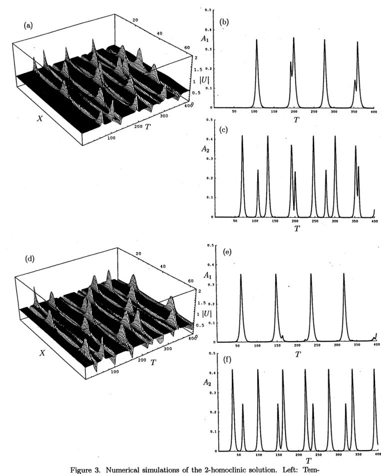
Next, a -homoclinic solution is investigated by an initial condition

$V=0.5\{1+\epsilon_{1}\exp(i\varphi i1)\cos[p_{1}(X-X1)]+\epsilon_{2}\exp(i\varphi i2)\cos[p_{2}(x_{-}X_{2})]\},$ (25)

with $p_{1}=2\pi/L=p_{2}/2,$ $X_{1}=0,$ $L=4\sqrt{2}\pi$ and $\epsilon_{1}=\epsilon_{2}=10^{-15},$ _{$X_{2}=0$}

for one case and $\epsilon_{1}=\epsilon_{2}=10^{-8},$ _{$X_{2}=\pi/2$} for the other. A doubly-periodic

motion is observed numericallyinstead of the homoclinic solution. Following

the above argument on the temporal period,

we

may estimate the periods

between bumps as

$T_{\mathrm{P}^{i}}=-(\ln\epsilon i+\ln\epsilon_{f})/\Omega_{i}$ (26)

Then, the ratio of the two periods is determined by the ratio of the linear

growth rates as

(6)

The present example gives $\Omega_{1}=\sqrt{7}/8,$$\Omega_{2}=1/2$ and $\nu--0.661$ and the

numerically obtained values are$T_{p1}=84,$$T_{p2}=57$and $\nu=0.679$. Therefore,

the theoretical prediction is confirmed by this numerical simulation.

A generalized homoclinic solution ofthe NLS equation is given and it is

shown that it appears as periodic and quasi-periodic motions in numerical

simulations with minimized numerical errors. The dependenceofthe period

on the magnitude of errors may not be restricted to this example but is

expectedto be applicable to systems having homoclinic structures and small

perturbations or noise.

I thank Professor M. J. Ablowitz for his two seminars given in

Profes-sor Wadati’s group in Department of Physics, University of Tokyo, which

motivated me to study this subject.

References

[1] Ablowitz, M. J. and Herbst, B. M., SIAM J. Appl. Math. 50, 339 (1990).

[2] Ablowitz, M. J. and Ladik, J. F., Stud. in Appl. Math. 55, 213 (1976).

[3] Ablowitz, M. J., Schober, C. and Herbst, B. M., Phys. Rev. Lett. 71,

2683 (1993).

[4] Calini, A., Ercolani, N. M., McLaughlin, D. W. and Schober, C. M.,

Physica D89,227 (1996).

[5] Huta, A., Acta Fac. Rerum Natur. Univ. Comenian. Math. 2, 21 (1957).;

Lambert, J. D. Computational Methods in Ordinary $D$_,

ifferential

Equations

(John Wiley&Sons, 1973)

[6] McLaughlin, D. W. and Schober C. M., Physica D, 57,447 (1992).

(7)

Figure 1. Numerical

simulations of

the

1-homoclinic solution

(8)

$\mathrm{F}\mathrm{i}\mathrm{u}\mathrm{r}_{2}\mathrm{e}\mapsto_{||}^{2\mathrm{L}}|U_{1}+U-1|0^{\cdot}\mathrm{f}\mathrm{t}\mathrm{h}\mathrm{e}\mathrm{s}\mathrm{p}\mathrm{a}\mathrm{t}\mathrm{i}\mathrm{a}\mathrm{l}\mathrm{F}\mathrm{o}\mathrm{u}\mathrm{r}\mathrm{i}\mathrm{e}\mathrm{r}\mathrm{C}\mathrm{o}\mathrm{m}\mathrm{e}\mathrm{f}\mathrm{t}\cdot \mathrm{T}\mathrm{e}\mathrm{m}\mathrm{p}\mathrm{o}\mathrm{r}\mathrm{a}\mathrm{l}\mathrm{e}\mathrm{V}\mathrm{o}1\mathrm{u}\mathrm{t}\mathrm{i}\mathrm{o}\mathrm{n}\mathrm{o}\mathrm{f}\mathrm{p}\mathrm{o}\mathrm{n}\mathrm{e}\mathrm{n}\mathrm{t}_{\mathrm{S}}\tilde{U}\mathrm{l}\mathrm{a}\mathrm{n}\mathrm{d}\tilde{U}\mathrm{h}\mathrm{t}\mathrm{e}\mathrm{a}\mathrm{m}\mathrm{p}1\mathrm{i}\mathrm{t}\mathrm{u}\mathrm{d}\mathrm{e}A=-1$

.

Right: Plots of $({\rm Re}(V), {\rm Im}(V))$ at $X=0$

.

(9)

$T$

Figure 3. Numerical simulations of the -homoclinic solution. Left:

Tem-poral evolution of $|U|$ with double precision. Rght: Temporal evolution of

$A_{1}=\sqrt{|\tilde{U}_{1}|^{2}+|\tilde{U}-1|}$and $A_{\mathit{2}}=\sqrt{|\tilde{U}_{2}|^{2}+|\tilde{U}-\mathit{2}|}$. The initial condition is _$U=$

$0.5[1|\epsilon \mathrm{e}^{i\phi 0}1\cos p_{1}X+\epsilon \mathrm{e}^{i}\emptyset 02\cos p_{1}(X-x\mathit{2})],$ $L=4\sqrt{2}\pi,p_{1}=\mathrm{p}_{2}/2=2\pi/L$, and (a-c) $\epsilon=10^{-\mathrm{l}_{\backslash }})r,d\mathrm{v}_{2}=0$, (d-r) $\epsilon=10^{-\hslash},\mathfrak{l}^{\gamma}2\Delta \mathrm{Y}2=\pi/2$