博士論文、修士論文 watanabe dthesis v4

(1)

Spectral Study of Stellar Winds Interacting with

X-rays from Accreting Neutron Stars

Shin Watanabe

Department of Physics

Graduate School of Science

University of Tokyo

(2)

Abstract

We have observed two archetype high mass X-ray binaries (HMXBs), Vela X-1 and GX 301₋2, with the Chandra _{grating spectrometer HETGS. By using the instrument}

with high energy resolving power E/∆E _∼ 100–1000, we perform precise measurements of various emission lines and spectral features in their X-ray spectra. In the case of Vela X-1, emission lines from highly ionized ions driven by photoionization, in addition to fluorescent lines from ions in various charge states, are clearly detected. The intensities and the centroid energies of these lines are determined with the highest accuracy ever achieved for this source. In the case of GX 301₋2, fluorescent emission lines are observed without any signature associated with highly ionized ions. Additionally, the Compton scattered line profile (Compton shoulder) is discovered in the intense iron Kα line of GX 301₋2, for the first time from a celestial source. In order to deal with such new probes, we have developed the simulator on the basis of Monte Carlo methods. By adopting this simulator to Vela X-1, we can find the ionization structure and the matter distribution, which reproduce the observed line intensities and continuum shapes. Additionally, from the amount of the Doppler shift due to the stellar wind velocity, we show that the stellar wind flow is affected by the photoionization by the neutron star radiation. For GX 301₋2, we have demonstrated that Compton shoulders could become a new probe to diagnose the physical conditions of cold material. In fact, we have found that a cold (<3 eV) and dense (NH ∼ 1024 cm−2) cloud is surrounding the neutron star almost spherically from

(3)

Chapter 1 Introduction

In high mass X-ray binary (HMXB) systems, the neutron star captures the surrounding material of the stellar wind from the massive hot star, and converts it into X-ray radi-ation. This emission interacts with the stellar wind, resulting in various emission lines and characteristic features in the X-ray spectrum. Because these structures are directly connected to the physical state of the material, the precise measurement brought by the high precision X-ray spectroscopy can provide essential information on the physical conditions and geometry of the matter in the vicinity of the neutron star.

Chandra _and XMM-Newton _{ray satellites have opened up a new dimension for}

X-ray spectroscopic observations, in the 21st century. The grating instruments on board

Chandra _and XMM-Newton _{have 10–100 times more improved energy resolving powers}

than that of past instruments. A number of forested emission lines, which were formerly seen as one broad line, can be fully-resolved individually. Additionally, hidden structures can be observed and clearly measured without any ambiguities.

HMXB observations using these grating instruments allow us to study the structure of stellar winds by the individual emission line from various ions, and, for the first time, provide a dynamical view of the ionized stellar wind surrounding the neutron star. At the same time, such observations also provide numerous difficulties that cannot be explained in the terms of simple models such as a spherically symmetric geometry or uniform density. Therefore, for capitalizing on the observation results and further understanding the information contained, new analytical methods and calculations are needed.

In this thesis, we deal with two different archetypes of high mass X-ray binaries, Vela X-1 and GX 301₋2. The former has highly ionized gases while the latter is characterized by heavy absorption and absence of any features connected with highly ionized ions. We have observed these two HMXBs with the grating spectrometers on Chandra_{, and, have}

obtained X-ray spectra with high precision. In order to analyze these X-ray spectral features and investigate the physical nature and geometry of the material, we have newly constructed a simulator on the basis of Monte Carlo methods.

(6)

(7)

Chapter 2 High Mass X-ray Binaries and X-ray

Spectroscopy

2.1 High Mass X-ray Binaries

A high mass X-ray binary (HMXB) is a system consisting of a neutron star or a black hole and a massive O- or B-type companion star. OB stars, which are young giant stars, have powerful stellar winds and are spreading a fraction of their mass continuously. A neutron star is a compact high-density object with a mass of _∼ 1.4 M¯ and a radius of

∼ 10 km. As it revolves around the companion star, it sweeps up the matter transfered by the stellar wind. When the matter is accreted on the neutron star, a fraction of its gravitational potential energy is converted into X-ray radiation. They are among the brightest X-ray sources in our galaxy and have been observed since the early days of X-ray astronomy.

X-ray emission from the neutron star in HMXBs have several interesting features; pulsation sometimes detected with a period of one to several hundred seconds and cy-clotron absorption structures in the hard X-ray spectra (Mihara, Makishima, & Nagase 1998; Makishima et al. 1999). These features are connected with the accretion and the strong magnetic field of the neutron star.

(8)

2.2 X-ray Spectroscopic Observations of HMXBs

2.2.1 Iron emission line and absorption edge

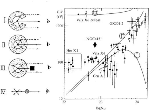
Since the early days of X-ray astronomy, emission lines and absorption edges of iron have played important roles for probing the matter distribution in HMXBs. The gas scintillation proportional counter (GSPC) on board Tenma satellite demonstrated the importance of the spectroscopic study of plasmas by using the most abundant material ions. With Tenma observations of several HMXBs, the emissions lines at 6.4 keV and the K-edge absorption features of iron ions in a low ionization degree have been shown in their X-ray spectra (e.g. Vela X-1 Ohashi et al. 1984; Nagase et al. 1986; GX 301₋2 Makino 1985; see Figure 2.1).

Figure 2.2 shows the iron line intensity plotted against the absorption-corrected con-tinuum intensity above the iron K edge energy. The proportional relation between these two values and the observed energy of the line center indicates that the iron line from HMXBs is produced through fluorescence of continuum X-rays by cold material.

The matter distribution around X-ray sources were estimated from the relations be-tween the line equivalent widths and the absorption column densities obtained from the continuum shape (Koyama 1985; Inoue 1985; Makishima 1986). Figure 2.3 shows the relation between these two values calculated by Monte Carlo method for some models of matter distributions, together with observed values for HMXBs and other X-ray sources. The pictures inferred with Tenma in the 1980s have been confirmed by ASCA in the 1990s. Additionally, the X-ray CCD on board ASCA is capable of investigating energy shifts and broadenings of the iron Kα line (Endo et al. 2002). However, the energy resolving power had not reached the level to recognize quantum effects, which is directly connected to the physical state of the matter.

2.2.2 Emission lines from lighter elements

(9)

Figure 2.1: Energy spectrum of Vela X-1 (left) and that of GX 301₋2 (right) obtained with Tenma. ((left) From Nagase et al. 1986, (right) From Leahy et al. 1989)

(10)

Figure 2.3: Relation between the matter thicknessNHand the iron line

(11)

same time from the source. Subsequently, Liedahl & Paerels (1996) and Kawashima & Kitamoto (1996), for the first time, detected a narrow radiative recombination continuum (RRC) of S XVI in ASCA spectrum of Cyg X-3, which provided evidence that the plasma in Cyg X-3 is ionized through photoionization, and the highly ionized gas in the plasma makes emission lines in the X-ray spectrum.

The spectral resolutions (E/∆E _∼100–1000) of diffraction grating spectrometers on board Chandra and XMM-Newton have a pottential to provide an unambiguous infor-mation of narrow RRCs in HMXBs. Paerels et al. (2000) resolved narrow RRCs of Si XIV and S XVI in the spectrum of Cyg X-3 with Chandra HETGS, and measured the electron temperature,kTe∼50 eV. Schulz et al. (2002) detected a narrow RRC from Ne

X with an electron temperature of _∼ 10 eV in the Chandra HETGS spectrum of Vela X-1. These observations have revealed that the photoionization-driven plasma indeed exists in HMXBs.

(12)

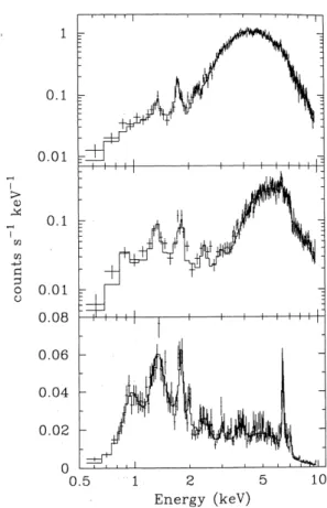
Figure 2.4: Energy spectra of Vela X-1 obtained with ASCA SIS at (top) posteclipse, (middle) pre-eclipse, and (bottom) eclipse phases during the or-bital phase intervals of 0.11 to 0.15, ₋0.14 to ₋0.11, and ₋0.10 to 0.10, respectively. (From Nagase et al. 1994)

(13)

Figure 2.6: The energy spectrum of Vela X-1 at the eclipse phase obtained with ASCA SIS and the model generated by Sako et al. (1999).

Stellar Wind

Companion Star

（O,B super-giant）

Neutron

Star

Scattering

Absorption

Photo Ionization

Recombination

X-ray

(14)

2.3 Basic Physical Processes in High Mass X-ray

Bi-naries

2.3.1 Stellar winds of OB super-giant stars

Winds ejected from hot stars such as O-stars and B-supergiants, are characterized by two global parameters, the terminal velocity v∞ and the mass loss rate ˙M∗. These

winds are initiated and then continuously accelerated by the radiation pressure on ions with resonance lines in the ultraviolet region. The velocity of the wind reaches to the maximum, v∞ at very large distances from the star, where the radiative acceleration

approaches zero.

Castor, Abbott & Klein (1975) and Pauldrach, Puls & Kudritzki (1986) showed that the velocity of the stellar winds obey the approximate formula (CAK-model):

v(r) =v∞

µ

1₋ R∗ r

¶β

(2.1)

for a given distancerfrom the center of the star, whereR∗is the stellar radius. Pauldrach,

Puls & Kudritzki (1986) show that the value of β _∼ 0.8 is a better representation of the wind kinematics for isolated OB stars. From the observational point of view, v∞ and β

can be determined from the analysis of the “P Cygni” profile which appears in the UV resonance line spectrum, and are actually obtained from many OB-stars. (e.g. Howarth & Prinja 1989; Prinja et al. 1990; Blomme 1990)

Given the velocity profile, the wind density can be calculated by applying the equation of mass continuity, assuming spherical symmetry:

n(r) = M˙∗ 4πµmpv(r)r2

, (2.2)

whereµis the gas mass per hydrogen atom. (µ= 1.3 for the cosmic chemical abundance.)

2.3.2 Capture of the stellar wind by the neutron star

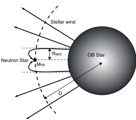
In the case of high mass X-ray binary systems consisting of a neutron star and an OB star, mass accretion onto the neutron star takes place through direct capture of the stellar wind material. Material within a radius Racc will be accreted by the gravitation

of the neutron star, whereas material outside this cylinder will escape (Figure 2.8). This radius is calculated by a simple assumption that material will be accreted only if it has a kinetic energy less than the potential energy in the vicinity of the neutron star. When the neutron star mass is quoted as Mns, it is set by

1 2mv

2 rel=

GMnsm

Racc

(15)

Racc Neutron Star D OB Star Stellar wind Mns

Figure 2.8: Geometry of accretion onto a neutron star.

for a particle of mass m. This relation gives

Racc =

2GMns

v2 rel

, (2.4)

wherevrel is the relative velocity of the neutron star and the stellar wind. Therefore, the

mass accreting rate onto the neutron star ˙Macc is given by

˙ Macc =

˙ M∗R2_acc

4D2 =

(GMns)2M˙∗

v4 relD2

, (2.5)

where D is the distance of the neutron star from the center of the OB star.

The gravitational energy of the accreting material is converted into rays. The X-ray luminosity resulting from this accretion will simply be the rate at which gravitational energy is released:

Lx =

GMnsM˙acc

Rns

= (GMns)

3 _˙ M∗

Rnsv_rel4 D2

(2.6)

where it is assumed that most of this energy is liberated near the neutron star surface (of radiusRns). By applying typical parameters (Mns= 1.4M¯,M˙∗ = 1×10

−6_M

¯ yr −1_{, R}

ns=

10 km, vrel = 500 km s

−₁

, D = 50R¯), we obtain a typical X-ray luminosity of HMXB,

Lx ∼5×1036 erg s−1.

(16)

the postshock accretion region (Lamb & Sanford 1979; Sunyaev & Titarchuk 1980; Becker & Begelman 1986). Kretschmar et al. (1997) applied these models to the spectrum of Vela X-1 obtained by HEXE on the RXTE satellite and TTM on MirKvant space station. They concluded that the power-law with an exponential cutoff model generally provides the best representation to the observed spectra. As the extension of the Comptonization models, on the other hand, Mihara, Makishima, & Nagase (1998) proposed a new model with a electron cyclotron resonance absorption feature, and claimed that the model pro-vides a better representation for the spectra of HMXBs obtained with Ginga. These analysis of cyclotron resonance absorptions results in the surface magnetic field of the neutron stars of a few times 1012 _G.

2.3.3 Photoionized plasmas

Strong X-ray radiation from the neutron star affect on the ionization and thermal struc-ture of the surrounding gas. The plasma surrounding the X-ray source is ionized and heated through photoionization and loses energy mainly through cascades following radia-tive recombination. Both the equilibrium temperature and the charge state distribution in this photoionized plasma are determined locally by the X-ray flux, the X-ray spectral shape and the gas density, and are often characterized by the ionization parameter,

ξ = LX ner2

, (2.7)

where LX is the luminosity of the X-ray source, ne is the electron density of the region,

and r is the distance to the X-ray source (Tarter, Tucker & Salpeter 1969).

(17)

The principal distinction between collisionally ionized and photoionized plasmas is the very different electron temperatures that accompany a given charge state distribution. For collisional ionization, the electron temperature must be comparable to the ionization potential, whereas for photoionization, the X-ray radiation does most of the work, so the electron temperature can be much lower. The most useful spectral diagnostic for observationally distinguishing between the two cases is the radiative recombination con-tinua. Descriptions of the radiative recombination continua are given in the following subsections.

2.3.4 Interactions between X-ray photons and photoionized

plas-mas

The physical processes in photoionized plasmas can be summarized.

Photoionization and Radiative Recombination

In the energy region of X-rays, the dominant process by which photons lose energy is photoionization. This process can be written as

Xi+γ −→X(

∗) i+1+e

−

,

where Xi represents an ion in charge state i (i.e. of ion Xi+), and an asterisk denotes

an ion in an excited state, while a parenthesized asterisk refers to an ion in either an excited state or the ground state. If the energy of the incident photon is E, it can eject electrons, which have binding energies Ebinding ≤E from atoms, ions and molecules, the

remaining energy (E₋Ebinding) being removed as the kinetic energy of the ejected electron.

The energy levels within the atom for which E =Ebinding are called “absorption edges”

because ejection of electrons from these energy levels is impossible if the photons have lower energy. For photons with higher energies, the cross section for photoionization from this level decrease roughly asE−3_{. There is an analytic solution for the photoionization}

cross section for photons with energies E _ÀEbinding and E ¿ mec2 due to the ejection

of electrons from the K-shells of H-like ions,

σK= 2

√

2σTα4Z5

µ

mec2

E

¶72

(2.8)

In this cross section,αis the fine structure constant andσTis the Thomson cross section.

There is the strong dependence of the cross section on the atomic number Z. Therefore, although heavy elements are very much less abundant than hydrogen, rare large-Z ele-ments make important contributions to the photoionization cross section.

Photoionization is balanced by its inverse process, radiative recombination,

Xi+e−1 −→X(

(18)

(19)

The photons generated in recombination are distributed into a continuum, the radiative recombination continuum (RRC), which is found above the recombination edge with a width ∆E _≈ kTe. In photoionized plasmas with a low electron temperature, the

RRC feature is narrow, and appears “line-like”. The emission coefficient for radiative recombination is given by

ji(E)dE =nevσP Ii (v)f(v)dv (2.9)

where ne is the electron density, v is the velocity of the free electron, and f(v) is the

Maxwellian velocity distribution,

f(v) = √4

π

µ

me

2kTe

¶3/2

v2exp

µ

−mv

2

2kTe

¶

. (2.10)

σP I

i (v) is the photoionization cross section, and

E = 1 2mev

2₊_E

i, (2.11)

whereEi is the ionization potential energy of leveliof the ion. To date, in X-ray regions,

the only identified RRC features have been associated with recombination to the ground level of H-like and He-like ions, but more often recombination leaves an ion in an excited state.

Subsequent to recombination into an excited level, the ion will decay in a series of spontaneous radiative transitions, until it reaches the ground level.

X∗

i −→Xi+γ

These radiative transitions generate photons whose energies are identified with the source ions, and form the emission line.

Fluorescence

Fluorescence line emission is also important process in photoionized plasmas, especially for ions in a low charge state. A photon ionizes an inner-shell electron of an ion in the ground state and leaves the ion in an excited state. One of the two following processes can occur at this point. The ion can stabilize itself through either, ejection of one or more Auger electrons, or emission of a photon. These processes can be described by the following,

Xi+γ −→Xi∗+1+e

−

−→

(

Xi+1+e−+e′− (Auger) Xi+1+e−+γ′ (fluorescence)

The probability of producing a fluorescent line instead of emitting Auger electrons is called the fluorescent yield, which increases as the atomic number. Fluorescent yields of neutral atoms for K and L shells are shown in Figure 2.10. For example, the fluorescent yield YK of the Kα line of iron at 6.4 keV is 0.30. For the Si Kα line at 1.74 keV, YK is

(20)

Figure 2.10: Fluorescent yields for K and L shells for 5 _≤ Z _≤ 110. (From X-RAY DATA BOOKLET(http://xdb.lbl.gov/))

Photoexcitation

Photoexcitation occurs when a photon excites a bound state of an ion, and is followed by a radiative decay resulting in an emission of a photon.

Xi+γ −→Xi∗ −→Xi+γ′

In the X-ray region, photoexcitations due to H-like and He-like ions of C, N, O, Ne, Mg, Si and so on play important roles on both emission and absorption line formations.

The cross section of photoexcitations from level i to level j (j > i) depends directly on the oscillator strength of the transition between leveli and j (fij), and is given by,

σP E_ij (E) =

√

πe2 mec2

fij

∆νD

H(a, x),

where H(a, x) is a Voigt function,

H(a, x) = a π

Z ∞

−∞

e−t2

dt

(x₋t)2₊_a2. (2.12)

In these equations,a=Ar/(4π∆νD),Aris the radiative decay rate, andx= (ν−νij)/∆νD

is the frequency shift from the line center expressed in units of the Doppler width,

∆νD =νij

r

2kT mzc2

(21)

Radiative recombination

Photoexcitation

Fluorescence

Photoionization

(22)

Compton Scattering

Compton scattering is a fundamental physical process that is responsible for transferring energy between photons and electrons in a wide variety of astrophysical environments. Since the Compton scattering opacity relative to that of photoionization is larger for higher energy photons, it plays an important role in the hard X-ray region. When a pho-ton propagating through a material undergoes Comppho-ton scattering with the constituent electrons, the energy of photon is modified in a way that depends on the scattering an-gle, the electron velocity and the electron state, whether it is bound or free. In the limit where the electrons are free and at rest, a fraction of the photon energy is transferred to the electron according to the Compton formula,

E1 =

E0

1 + (E0/mec2) (1−cosθ)

, (2.14)

or,

cosθ = 1₋mec2

µ

1 E1 −

1 E0

¶

(2.15)

whereE0 is the energy of the incoming photon,E1 is the energy of the outgoing photon, θ is the angle between the incoming and outgoing photons, andmec2 is the electron

rest-mass energy (=511 keV). The differential cross section for unpolarized photons is shown in quantum electrodynamics to be given by the Klein-Nishina formula

dσ dΩ =

r2 0 2 E2 1 E2 0 µ E0 E1

+E1 E0 −

sin2θ

¶

. (2.16)

The total cross section can be shown to be

σ=σT·

3 4

·

1 +x x3

½

2x(1 +x)

1 + 2x −ln (1 + 2x)

¾

+ 1

2xln (1 + 2x)−

1 + 3x (1 + 2x)2

¸

(2.17)

where x=E0/mec2 and σT is Thomson cross section.

2.3.5 X-ray emission lines from photoionized plasmas

From hydrogen like ions

The most prominent emission lines from H-like ions are the Lyman series transitions:

Lymanα1,2 : 2p 2P3/2,1/2 −→1s 2S1/2

Lymanβ1,2 : 3p 2P3/2,1/2 −→1s 2S1/2

Lymanγ1,2 : 4p 2P3/2,1/2 −→1s 2S1/2

(23)

Figure 2.12: A model of emission lines from H-like Si.

In photoionized plasmas, Lyman series lines are formed by radiative decays following either photoexcitation or radiative recombination. The energies of these lines can be calculated precisely from theory. Therefore, observed profiles of the lines such as widths and energy shifts enable us to investigate the dynamics of the emission site.

The RRC feature becomes narrow, and appears the line-like profile due to the low electron temperature of the photoionized plasma. Additionally, the width of the RRC corresponds to directly electron temperature of the recombination site. A model of X-ray emission lines from H-like Si is shown in Figure 2.12.

From helium like ions

The most important K-shell He-like transitions are as follows:

(24)

The line w is an electric dipole transition, also called the resonance transition, and is sometimes designated with the symbolr. Linesxandyare the so-called intercombination lines. These are usually blended and are collectively designated with the symboli. Lastly, z is the forbidden line, often designated by the symbol f. Emissions from He-like ions are characterized with the triplet lines of r, i and f.

In photoionization plasmas, as in the H-like case, the excited levels for He-like ions are fed directly by photoexcitation and radiative recombination. The three He-like lines ratios can be affected by the electron density and the presence of a significant ultraviolet radiation field. The density sensitivity comes from the fact that the 3S1 level can be

collisionally excited to the 3_P _{levels. At high-enough electron density, this process}

suc-cessfully competes with radiative decay of the forbidden line. In the UV radiation field,

3_S

1 level can be also excited to 3P levels by photoexcitation. These lead to suppression

of the forbidden line and enhancement of the intercombination lines. Additionally, inner-shell ionization of Li-like ions can lead to the production of the forbidden line in He-like ions. Despite its use as density, temperature and UV radiation diagnostics, the behavior of the triplet lines ratios from He-like ions is very complex.

The transition energies of He-like ions can also be determined accurately from the-oretical calculations. The energy shift of the observed line from the calculated value is available for study of dynamics. The RRC feature also appears in the same way as that of H-like ions. A model of emission lines from He-like Si is shown in Figure 2.13.

From ions in a low charge state

Fluorescent line emission from ions in a low charge state is another important line for-mation process in photoionized plasmas. An intensity of a fluorescent emission is propor-tional to the fluorescent yield (_§2.3.4), which increases as the atomic number. Therefore, an emission line from a fluorescence of a high-Z element like iron becomes appreciable.

The energy of the fluorescent emission is affected by the charge state of the ion, and behaves intricately. Therefore, in comparison to emission lines from H-like and He-like ions, it is complex for study of dynamics to utilize fluorescent lines.

Compton shoulder

As described in _§ 2.3.4, when an X-ray photon propagating through a low-temperature (<105 _{K) medium undergoes Compton scattering with the constituent electrons, a}

frac-tion of the photon energy is is transferred to the electron according to the Compton formula (eq. 2.14, 2.15). The maximum energy shift per scattering due to the electron recoil is, therefore,

∆Emax=

2E2 0 mec2+ 2E0

, (2.18)

for photons that are back-scattered (θ = 180◦

(25)

(26)

(τCompton >0.1) has a non-negligible probability of interacting with an electron, resulting

in down-scattering of photons and, hence, producing a discernible ”Compton shoulder” betweenE0 andE0−∆Emax. Alternatively, this Compton energy shift can be written in

wavelength form:

∆λmax=

hc

E0−∆Emax − hc E0

= 2h mec

= 2λC, (2.19)

where λC =h/mec∼ 0.024 ˚A is Compton wavelength. Therefore, the maximum

wave-length shift due to Compton scattering is constant independent of the incident energy. X-ray emission lines at higher energies are ideal for studying the properties of the Compton shoulders, since the Compton scattering opacity relative to that of photoion-ization is larger for higher energy photons. The iron Kα fluorescent line complex at E0 = 6.40 keV, therefore, is particularly promising, and can be produced over an

ex-tremely wide range in column density, which makes it ideal for diagnosing the physical properties of a cold medium irradiated by X-rays. The energy shift of an iron line photon due to a single Compton scattering is 156 eV from eq. (2.18).

(27)

(28)

Chapter 3 Instrumentation

In this thesis, we utilize observational data obtained with the grating spectrometer on board the Chandra _{X-Ray Observatory. In this chapter, we summarize the basic}

proper-ties and performance of the satellite and the instruments.

3.1 Chandra Observatory

The Chandra _{X-Ray Observatory was launched by} NASA_{’s Space Shuttle Columbia on}

July 23, 1999. The schematic view of the satellite is shown in Figure 3.1. The Chandra

satellite carries a high resolution X-ray mirror, two imaging detectors, and two sets of transmission gratings. The important features are: an order of magnitude improvement in spatial resolution, and the capability for high spectral resolution with the gratings.

The X-ray mirror, High Resolution Mirror Assembly (HRMA), consists of a nested set of four paraboloid-hyperboloid (Wolter-1) grazing-incidence X-ray mirror pairs. It achieves an excellent angular resolution of 0.5′′

(29)

Figure 3.1: A schematic view of Chandra satellite. The satellite is more than 10 m long and weights about 5 tons. The satellite is thrown into an elliptical high-Earth orbit with the perigee altitude of 10,000 km, the apogee altitude of 140,000 km, with the orbital period of about 64 hours.

3.2 High Energy Transmission Grating

Spectrome-ter(HETGS)

3.2.1 HETGS overview

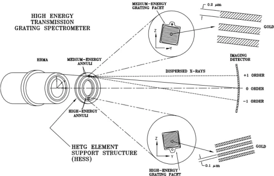
The HETGS provides high resolution spectra (withE/∆E up to 1000) between 0.4 keV and 10.0 keV for point and slightly extended (few arc seconds) sources. The HETGS consists of two sets of gratings, each with different period. One set, the Medium Energy Grating (MEG), is optimized for medium energies. The second set, the High Energy Grating (HEG), is optimized for high energies. The HETG is designed for use with the spectroscopic array of the Chandra _{CCD Advanced Imaging Spectrometer (ACIS-S).}

A schematic layout of the HRMA-HETG-detector system is shown in Figure 3.2. X-rays from the HRMA strike the transmission gratings and are diffracted by an angle β given according to the grating equation,

sinβ =mλ/p, (3.1)

(30)

Figure 3.2: A schematic layout of the High Energy Transmission Grating Spectrometer. (from The Chandra Proposers’ Observatory Guide)

Figure 3.3: A HETGS raw image.

primarily the first-order, _|m_| = 1. MEG has a period of 4001.41 ˚A and HEG has a period of 2000.81 ˚A. The two sets of gratings are mounted with their rulings at different angles so that the dispersed images from the HEG and MEG form a shallow “X” like image centered on the undispersed (zeroth order) position: one leg of the “X” is from the HEG, and the other from the MEG (Figure 3.3).

3.2.2 HETGS performance

(31)

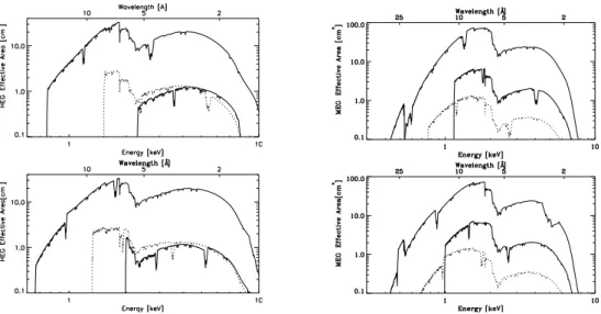
Figure 3.4: The HETGS effective area, integrated over the Point Spread Func-tion (PSF), is shown with energy and wavelength scales. The two panels in the left side show HEG effective areas, and the two panels in the right side show MEG effective areas. The m = +1,+2,+3 orders are displayed in the top panels and m = ₋1,₋2,₋3 orders are in the bottom panels. The thick solid lines are first order, the thin solid lines are third order, and the dotted lines are second order. (from The Chandra Proposers’ Observatory Guide)

energy, described as an “ancillary response file” or ARF_{. Effective area of HEG and}

MEG extracted from nominal HETGS ARF_{’s are shown in Figure 3.4. Based on the}

results from the HETGS calibration observations, the systematic uncertainties of HETGS spectral fluxes are estimated as follows,

• 10 % for 1.5 <E < 6 keV (both MEG and HEG)

• 20 % for 6< E <8 keV (HEG only)

• 20 % in the Si-K edge region (1.83–1.84 keV) (both MEG and HEG)

• 20 % for 0.8 <E < 1.5 keV (both MEG and HEG)

• 30 % for 0.5 <E < 0.8 keV (MEG only).

(32)

Figure 3.5: HEG and MEG Resolving Power (E/∆E=λ/∆λ) as a function of energy for the nominal HETGS configuration. The ”optimistic” dashed curve is calculated from pre-flight models and parameter values. The ”conservative” dotted curve is the same except for using plausibly degraded values of aspect, focus, and grating period uniformity. The cut-off at low-energy is determined by the length of the ACIS-S array. Measurements from the HEG and MEG m = ₋1 spectra, are typical of flight performance and are shown here by the diamond symbols. The values plotted are the as-measured values and therefore include any natural line width in the lines; for example, the ”line” around 12.2 ˚A is a blend of Fe and Ne lines. (from The Chandra Proposers’ Observatory Guide)

The wavelength resolution ∆λ is written as

∆λ= p

mcosβ∆β, (3.2)

according to eq.(3.1). For smallβ, the resolution is independent ofλ for a fixed telescope angular resolution ∆β. The resolving power,E/∆E =λ/∆λ, of HETGS are shown with respect to the energy of incident photons in Figure 3.5. The ∆λs (FWHM) are 0.012 ˚A and 0.024 ˚A for HEG and MEG, respectively. Therefore, the energy resolutions of HEG are 4 eV at 2 keV and 40 eV at 6.4 keV.

(33)

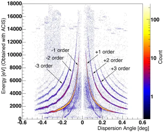
Figure 3.6: A HEG event distribution in dispersion angle/energy obtained from CCD pulse height space. Each order events can be seen.

3.3 Data Process

When we observe an X-ray source with HETGS, we obtain a dispersed image such as raw data (Figure 3.3). By using the image, we can select dispersed events of MEG and HEG on the basis of spatial positions. And then, we use an order sorting mask by using the energy information obtained with ACIS. Figure 3.6 shows a distribution of events in the dispersion angle/CCD pulse height space. Dispersion angles are converted from the distance from the center point of the zeroth order image. As shown in Figure 3.6, events of each order are clearly separated. In the data analysis, we first select events of the intended order, and then, extract a spectrum by projecting the events on dispersion angle axis. Finally, by converting the dispersion angle into wavelength or energy on the basis of eq.(3.1), we obtain a wavelength spectrum or an energy spectrum.

(34)

Chapter 4 Observations and Results of

Vela X-1

4.1 Vela X-1

Vela X-1 is an eclipsing high mass X-ray binary pulsar with a pulse period of 283 s (McClintock et al. 1976) and an orbital period of 8.964 days (Forman et al. 1973). The optical companion star, HD 77581, is a B05 Ib supergiant (Brucato & Kristian 1972; Hiltner, Werner & Osmer 1972), which drives a stellar wind with a mass-loss rate of (1– 7)_×10−6_M

¯yr

−1_{(Hutchings 1976; Dupree et al. 1980; Kallman & White 1982; Sadakane}

et al. 1985; Sato et al. 1986a). The 1100 km s−1 _{terminal velocity of the stellar wind was}

measured by Prinja et al. (1990) from the P-Cygni profile of the UV resonance line. Its intrinsic X-ray luminosity is _∼ 1036 _{erg s}−1_{, consistent with accretion of a stellar wind}

captured by the neutron star gravitation for the mass-loss rate and the velocity structure (see Chapter 2).

Neutron Star

Earth Eclipse

Phase 0.25

Phase 0.50 HD 77581

(35)

streak

Zeroth order HEG

MEG

Figure 4.2: The grating image of Vela X-1 in the phase 0.50.

4.2 Observation and Data Reduction

Chandra _{observed Vela X-1 three times. In order to observe from different places and}

to compare the results, we have planned to observe Vela X-1 at different orbital phases in the same orbit. The actually observed orbital phases are (1) φ = 0.237–0.278, (2) φ= 0.481–0.522, and (3)φ= 0.980–0.093, hereafter referred to as phase 0.25, phase 0.50, and eclipse, respectively. The observation dates and exposure times are summarized in Table 4.1.

All of the data are processed using CIAO v2.3, and spectral analyses are performed using XSPEC 1_{. Since the zeroth order image was severely piled-up (Figure 4.2) during}

phase 0.25 and phase 0.50, the locations of the zeroth order image were determined by finding the intersection of the streak events and the dispersed events. We apply spatial filters for both the MEG and the HEG, and then use an order sorting mask by using the energy information obtained with ACIS. In our analysis, only the first order events are used to extract spectra. The background events are estimated from the adjacent region to the dispersed event region. According to this estimation, the background levels are at most 5% for the eclipse data and 3% for phase 0.25 and phase 0.50 data.

The light curves in the three orbital phases extracted from the HEG in the energy interval between 1 and 10 keV (Figure 4.3). Pulsations with periods of 283.2 s and 283.5 s are found from the light curves of phase 0.25 and phase 0.50, respectively, by the epoch holding method. The HEG integrated spectra for each orbital phase are shown in Figure 4.4.

1

(36)

Table 4.1. Summary of Vela X-1 Observations

Label OBSID Start Date Orbital Phase Exposure (sec)

0.25 1928 2001-02-05 05:29:55 0.237 – 0.278 29570

0.50 1927 2001-02-07 09:57:17 0.481 – 0.522 29430

eclipse 1926 2001-02-11 21:20:17 0.980 – 0.093 83150

(37)

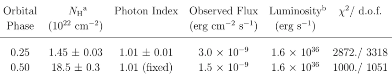
Table 4.2. Properties of continuum spectra derived from spectral fits.

Orbital NHa Photon Index Observed Flux Luminosityb χ2/ d.o.f.

Phase (1022 _cm−2₎ _{(erg cm}−2 _s−1₎ _{(erg s}−1₎

0.25 1.45 _± 0.03 1.01 _±0.01 3.0 _× 10−9 _1.6 _× ₁₀36 _{2872./ 3318}

0.50 18.5 _± 0.3 1.01 (fixed) 1.5 _× 10−9 _1.6 _× ₁₀36 _{1000./ 1051}

Note. — Fitting regions are 1.0–10.0 keV and 3.0–10.0 keV from HEG for 0.25 and 0.50 orbital phases, respectively. The iron K-line region (6.3–6.5 keV) is excluded. Errors correspond to 90 % confidence levels.

a_{The metal abundance is assumed to be 0.75 cosmic.}

b_{0.5–10.0 keV luminosity corrected for absorption.}

4.3 Continuum Emission

X-rays emitted from the neutron star are clearly observed from the spectra taken in phase 0.25 and phase 0.50, as featureless continuum spectra. As expected from the geometry, the spectrum taken in the eclipse phase is dominated by line emission and scattered components. In order to parameterize the properties of the continuum part of the spectra, we fit it with a photo-absorbed power-law function. Since the spectrum of phase 0.25 is less affected by absorption, we leave both the hydrogen column density and the photon index as free parameters in the fit. On the other hand, for phase 0.5, we fix the photon index to the value obtained from phase 0.25 and calculate the absorption. As for a metal abundance of the photo-absorption material, we use 0.75 times the cosmic chemical abundance (Feldman 1992), which is known to be representative for typical OB-stars (Bord et al. 1976). The derived parameters from the spectral fits are listed in Table 4.2. The best-fit models are superimposed on the spectra in Figure 4.4. The absorption-corrected luminosity is determined to be identical for observations in phase 0.25 and in phase 0.50 and corresponds to 1.6 _× 1036 _{erg s}−1 _{in the 0.5–10 keV range,}

assuming a distance of 1.9 kpc (Sadakane et al. 1985).

4.4 Emission Lines

(38)

(39)

detection and the identification of K-shell Si fluorescent lines from a wide range of charge state, for the first time from Vela X-1. The emission lines from highly ionized S, Si, Mg and Ne can be seen, in addition to fluorescent lines from Fe, Ca, S, and Si ions in lower charge states. Additionally, in the both spectra of phase 0.50 and eclipse, emission lines from the same ions are detected.

Blown-up spectra of the Si K lines region are shown in Figure 4.7. Intense Lyα line from H-like ions and fully-resolved He-like triplet lines are clearly seen in phase 0.50 and eclipse. At the lower energy end below 1.74 keV, fluorescent lines from near-neutral Si is also detected in both phases. Additionally, between the He-like lines and nearly neutral line, Si VII–Si XI Kα lines can be resolved. The forest of Si K lines is a clear evidence that plasma in various ionization states exist in the Vela X-1 system.

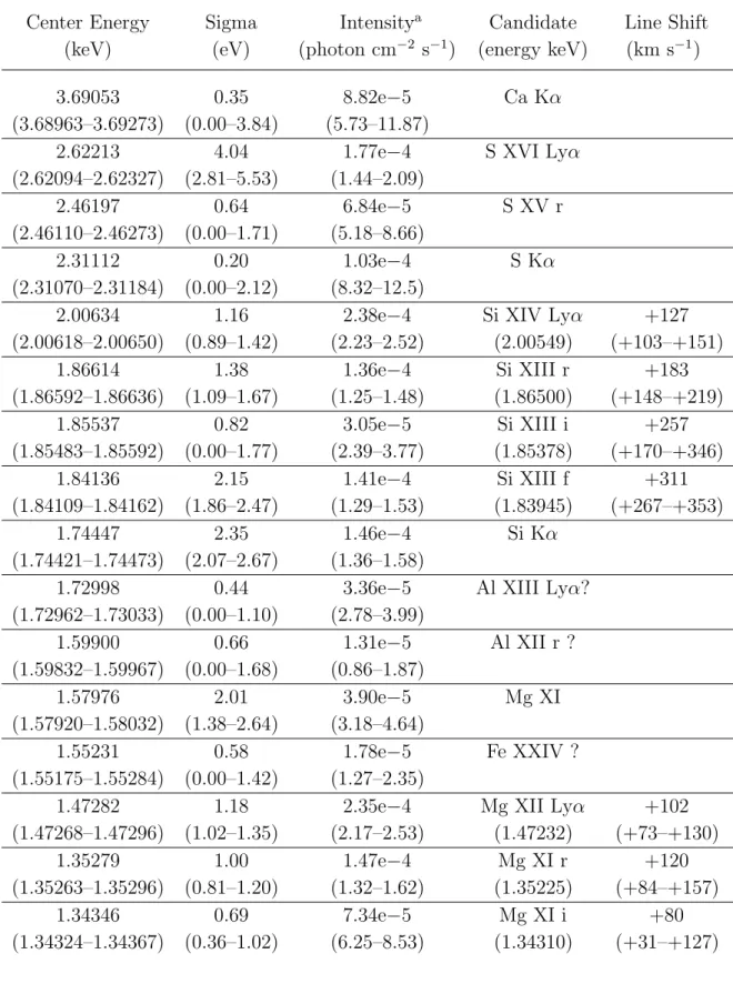
The centroid of energies, the widths and the intensities of each line are determined by fitting the data with a single gaussian model. In the spectral fittings, we use the Poisson likelihood statistics, in stead of the χ2 _{statisitics, because numbers of photons in some}

of the bins in the spectra are very small. As an example of the fittings, the Lyα line profiles from H-like ions of Si are shown in Figure 4.8, together with the best-fit models. The derived parameters for phase 0.50 and eclipse are listed in Table 4.3 and Table 4.4, respectively. The line intensity ratios of phase 0.50 to eclipse are listed on Table 4.5 for lines from H- and He-like ions which were detected with statistical significance of more than 5 σ. These ratios are 8–10 for the H-like lines and are 4–7 for the He-like lines.

One of the striking results seen from Figure 4.8 is the Doppler shift of lines. Thanks to the resolving power of the HEG, Doppler shifts can be measured with an accuracy of

∼ 100 km s−1_{. Figure 4.9 compares the line profiles of Si Ly}_α _{and Mg Ly}_α _{between the}

phase 0.50 and the eclipse data. The differences in the line center energies are clearly seen in each line.

In Figure 4.10, the velocity shifts are plotted for both of the phases for all emission lines from H- and He-like ions. Though some fluctuations are seen, there is a trend that blue shifts are detected in phase 0.50 and red shifts are observed in eclipse. The shifts between phase 0.50 and eclipse (∆v) range in_∼300–600 km s−1_{(Table 4.5). Additionally,}

the emission lines from highly ionized ions have widths of σ .300 km s−1_.

The radiative recombination continuum (RRC) is detected clearly from H-like Ne. The blow-up spectra of phase 0.50 and that of eclipse are shown in Figure 4.11. We fitted the RRC spectra using the “redge” model in XSPEC. The electron temperatures are derived to be kTe = 7.4+1−1..63 eV and kTe = 6.6+2−1..58 eV during phase 0.50 and eclipse,

respectively.

(40)

(41)

(42)

(43)

Si XIV Ly

α

Si XIII

r

f

i

Si II-VI

Si XI

Si X

Si IX

Si VIII

Si VII

phase 0.25

phase 0.50

eclipse

due to the detector

response (Si-Kedge)

(44)

(45)

Table 4.3. Derived Parameters of emission lines in the 0.5 orbital phase spectrum

Center Energy Sigma Intensitya _Candidate _{Line Shift}

(keV) (eV) (photon cm−₂

s−₁

) (energy keV) (km s−₁

)

3.69053 0.35 8.82e₋5 Ca Kα

(3.68963–3.69273) (0.00–3.84) (5.73–11.87)

2.62213 4.04 1.77e₋4 S XVI Lyα

(2.62094–2.62327) (2.81–5.53) (1.44–2.09)

2.46197 0.64 6.84e₋5 S XV r

(2.46110–2.46273) (0.00–1.71) (5.18–8.66)

2.31112 0.20 1.03e₋4 S Kα

(2.31070–2.31184) (0.00–2.12) (8.32–12.5)

2.00634 1.16 2.38e₋4 Si XIV Lyα +127

(2.00618–2.00650) (0.89–1.42) (2.23–2.52) (2.00549) (+103–+151)

1.86614 1.38 1.36e₋4 Si XIII r +183

(1.86592–1.86636) (1.09–1.67) (1.25–1.48) (1.86500) (+148–+219)

1.85537 0.82 3.05e₋5 Si XIII i +257

(1.85483–1.85592) (0.00–1.77) (2.39–3.77) (1.85378) (+170–+346)

1.84136 2.15 1.41e₋4 Si XIII f +311

(1.84109–1.84162) (1.86–2.47) (1.29–1.53) (1.83945) (+267–+353)

1.74447 2.35 1.46e₋4 Si Kα

(1.74421–1.74473) (2.07–2.67) (1.36–1.58)

1.72998 0.44 3.36e₋5 Al XIII Lyα?

(1.72962–1.73033) (0.00–1.10) (2.78–3.99)

1.59900 0.66 1.31e₋5 Al XII r ?

(1.59832–1.59967) (0.00–1.68) (0.86–1.87)

1.57976 2.01 3.90e₋5 Mg XI

(1.57920–1.58032) (1.38–2.64) (3.18–4.64)

1.55231 0.58 1.78e₋5 Fe XXIV ?

(1.55175–1.55284) (0.00–1.42) (1.27–2.35)

1.47282 1.18 2.35e₋4 Mg XII Lyα +102

(1.47268–1.47296) (1.02–1.35) (2.17–2.53) (1.47232) (+73–+130)

1.35279 1.00 1.47e₋4 Mg XI r +120

(1.35263–1.35296) (0.81–1.20) (1.32–1.62) (1.35225) (+84–+157)

1.34346 0.69 7.34e₋5 Mg XI i +80

(46)

Table 4.3—Continued

(keV) (eV) (photon cm−2 _s−1_{) (energy keV)} _{(km s}−1₎

1.33213 0.95 9.13e₋5 Mg XI f +230

(1.33190–1.33236) (0.65–1.25) (7.89–10.5) (1.33111) (+178–281)

1.30808 1.06 4.99e₋5 Fe XXI ?

(1.30766–1.30843) (0.61–1.49) (3.96–6.12)

1.27783 1.10 8.44e₋5 Ne X Lyγ

(1.27756–1.27811) (0.78–1.38) (7.18–9.84)

1.21160 0.94 1.33e₋4 Ne X Lyβ

(1.21139–1.21181) (0.72–1.17) (1.15–1.52)

1.12732 1.54 7.41e₋5 Ne IX

(1.12683–1.12780) (1.13–2.03) (5.71–9.27)

1.07432 0.12 5.76e₋5 Ne IX

(1.07397–1.07450) (0.00–0.73) (4.07–7.74)

1.02242 0.64 4.42e₋4 Ne X Lyα +182

(1.02230–1.02253) (0.52–0.76) (3.91–4.97) (1.02180) (+147–+214)

0.922458 0.80 2.89e₋4 Ne IX r +149

(0.922186–0.922725) (0.52–1.11) (2.24–3.64) (0.922001) (+60–+235)

0.916254 1.44 4.91e₋4 Ne IX i +475

(0.915937–0.916584) (1.21–1.73) (4.03–5.89) (0.914803) (+371–+583)

0.905561 1.78 3.71e₋4 Ne IX f +165

(0.905013–0.906071) (1.38–2.27) (2.88–4.65) (0.905062) (₋16–+334)

a_{Inter stellar gas absorption is corrected.} _{The hydrogen column density of}

6 _× 1021 _cm−₂

is assumed, corresponding to the density of 1 H cm−₃

and the distance of 1.9 kpc.

(47)

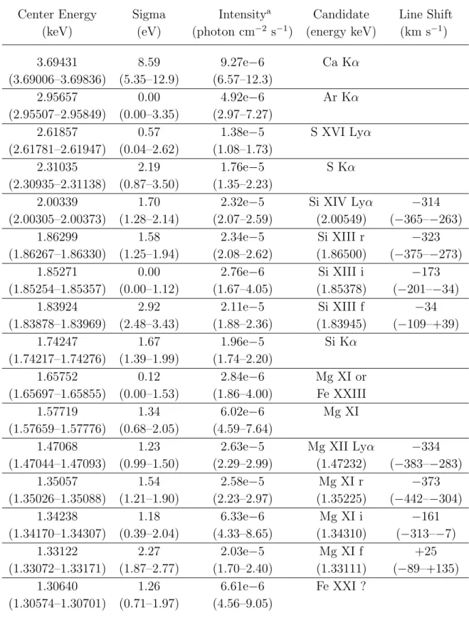
Table 4.4. Derived Parameters of emission lines in the 0.0 orbital phase spectrum

s−₁

) (energy keV) (km s−₁

)

3.69431 8.59 9.27e₋6 Ca Kα

(3.69006–3.69836) (5.35–12.9) (6.57–12.3)

2.95657 0.00 4.92e₋6 Ar Kα

(2.95507–2.95849) (0.00–3.35) (2.97–7.27)

2.61857 0.57 1.38e₋5 S XVI Lyα

(2.61781–2.61947) (0.04–2.62) (1.08–1.73)

2.31035 2.19 1.76e₋5 S Kα

(2.30935–2.31138) (0.87–3.50) (1.35–2.23)

2.00339 1.70 2.32e₋5 Si XIV Lyα ₋314

(2.00305–2.00373) (1.28–2.14) (2.07–2.59) (2.00549) (₋365–₋263)

1.86299 1.58 2.34e₋5 Si XIII r ₋323

(1.86267–1.86330) (1.25–1.94) (2.08–2.62) (1.86500) (₋375–₋273)

1.85271 0.00 2.76e₋6 Si XIII i ₋173

(1.85254–1.85357) (0.00–1.12) (1.67–4.05) (1.85378) (₋201–₋34)

1.83924 2.92 2.11e₋5 Si XIII f ₋34

(1.83878–1.83969) (2.48–3.43) (1.88–2.36) (1.83945) (₋109–+39)

1.74247 1.67 1.96e₋5 Si Kα

(1.74217–1.74276) (1.39–1.99) (1.74–2.20)

1.65752 0.12 2.84e₋6 Mg XI or

(1.65697–1.65855) (0.00–1.53) (1.86–4.00) Fe XXIII

1.57719 1.34 6.02e₋6 Mg XI

(1.57659–1.57776) (0.68–2.05) (4.59–7.64)

1.47068 1.23 2.63e₋5 Mg XII Lyα ₋334

(1.47044–1.47093) (0.99–1.50) (2.29–2.99) (1.47232) (₋383–₋283)

1.35057 1.54 2.58e₋5 Mg XI r ₋373

(1.35026–1.35088) (1.21–1.90) (2.23–2.97) (1.35225) (₋442–₋304)

1.34238 1.18 6.33e₋6 Mg XI i ₋161

(1.34170–1.34307) (0.39–2.04) (4.33–8.65) (1.34310) (₋313–₋7)

1.33122 2.27 2.03e₋5 Mg XI f +25

(1.33072–1.33171) (1.87–2.77) (1.70–2.40) (1.33111) (₋89–+135)

1.30640 1.26 6.61e₋6 Fe XXI ?

(48)

(keV) (eV) (photon cm−2 _s−1_{) (energy keV)} _{(km s}−1₎

1.27592 0.89 8.70e₋6 Ne X Lyγ

(1.27547–1.27636) (0.00–1.44) (5.62–11.4)

1.23618 1.57 5.94e₋6 Fe XX ?

(1.23507–1.23727) (0.71–2.79) (3.13–8.95)

1.20980 1.34 1.43e₋5 Ne X Lyβ

(1.20930–1.21033) (0.96–1.82) (1.07–1.84)

1.07241 0.78 1.91e₋5 Ne IX

(1.07205–1.07276) (0.44–1.19) (1.38–2.54)

1.02075 0.99 8.54e₋5 Ne X Lyα ₋308

(1.02056–1.02095) (0.81–1.18) (7.25–9.98) (1.02180) (₋364–₋249)

0.920773 0.92 5.48e₋5 Ne IX r ₋400

(0.920390–0.921159) (0.60–1.30) (3.86–7.43) (0.922001) (₋524–₋274)

0.914926 1.05 4.68e₋5 Ne IX i +40

(0.914407–0.915448) (0.75–1.53) (3.03–6.70) (0.914803) (₋130–+211)

0.904058 0.75 8.98e₋5 Ne IX f ₋333

(0.903784–0.904342) (0.48–1.10) (6.75–11.6) (0.905062) (₋424–₋239)

a_{Inter stellar gas absorption is corrected.} _{The hydrogen column density of}

6 _× 1021 _cm−2 _{is assumed, corresponding to the density of 1 H cm}−3 _{and the distance}

of 1.9 kpc.

Note. — Errors correspond to 90 % confidence level.

4.5 Pulse Phase Dependence

Figure 4.13 shows the pulse profiles at the orbital phase 0.25 and phase 0.50 obtained by folding the light curve of the 1–10 keV events from HEG _± 1 order. The pulse periods are 283.2 s and 283.5 s for phase 0.25 and phase 0.50, respectively. The pulse phase of 0.0 employed the barycentric start time of each observation. The observed pulse profiles are consistent with those reported in past observations; e.g. McClintock et al. (1976); Sato et al. (1986a); Kreykenbohm et al. (1999).

(49)

Figure 4.9: The line profiles of Si H-like Lyα (left) and Mg H-like Lyα. The blue lines show the observed data in phase 0.5, and the red lines show the data in eclipse. The HEG data is used for the Si Lyα lines, and the MEG data is used for the Mg Lyα lines.

(50)

Table 4.5. Comparison between lines of the phase 0.50 and of the eclipse.

line Intensity(0.50)/Intensity(eclipse) ∆v (km s−1₎

Si XIV Lyα 10.3 _± 1.3 441 _± 56

Si XIII resonance 5.81 _±0.83 506 _± 62

Si XIII forbidden 6.68 _±0.95 345 _± 86

Mg XII Lyα 8.94 _±1.37 436 _± 58

Mg XI resonance 5.70 _±1.00 493 _± 78

Mg XI forbidden 4.50 _±1.01 205 _± 123

Ne X Lyα 5.18 _±1.04 490 _± 60

Ne IX resonance 5.27 _±2.14 549 _± 153

Ne IX forbidden 4.13 _±1.49 498 _± 198

(51)

Table 4.6. Derived Parameters of the Fe Kα line.

Orbital Phase Center Energy Sigma Intensity EW

(keV) (eV) (photon cm−2 _s−1₎ _(eV)

0.00 6.3958 (6.3936–6.3980) 7.2 (1.9–11.1) 1.70e₋4 (1.50–1.90) 844 0.25 6.3992 (6.3987–6.4010) 0.0 (0.0–7.4) 1.92e₋3 (1.78–2.07) 51 0.50 6.3965 (6.3953–6.3976) 11.0 (9.1–12.8) 3.40e₋3 (3.21–3.58) 116

Note. — Only HEG data is used. The fitting model is single gaussian.

Note. — Errors correspond to 90 % confidence level.

(52)

Figure 4.13: Pulse profiles of Vela X-1 at orbital phase 0.25 (top panel) and 0.50 (bottom panel), obtained by folding the light curves at the barycentric periods of 283.2 s and 283.5 s, respectively. Two phase cycles are shown for clarity. The HEG_±1 order events are used, and the energy band is 1–10 keV. The pulse phase of 0.0 corresponds to the start time of each observation.

for each orbital phase, and Table 4.7 lists the observed fluxes and the corresponding iron Kα intensities.

Although the observed overall flux changes between the peak and the bottom by a factor of 1.3, the iron Kα line flux does not change within statistical uncertainty. Addi-tionally, the 1.0–2.1 keV count rate in orbital phase 0.50, dominated by Ne, Mg and Si emission lines, is constant between the peak and the bottom; specifically, 0.15_±0.01 c s−1

and 0.14 _± 0.01 c s−1 _{for the peak and the bottom, respectively.}

Table 4.7. Total and iron Kα fluxes of the pulse phase divided spectra

orbital Flux (1.0–10.0 keV)(erg s−₁

) Fe Kα flux (photon cm−₂

s−₁

)

phase peak bottom peak bottom

phase 0.25 (3.3 _± 0.1) _× 10−9 _(2.5 _± _0.1) _× ₁₀−9 _(1.8 _± _0.2) _×₁₀−3 _(2.1 _± _0.2) _× ₁₀−3

(53)

Figure 4.14: X-ray spectra divided by the pulse phase. The left panel shows spectra at orbital phase 0.25, and the right panel at orbital phase 0.50. Ma-genta and cyan spectra refer to the pulse peak and pulse bottom, respectively, as defined in Figure 4.13.

4.6 Summary of the Observation and the Implication

From the continuum spectral shapes, the direct radiation from the neutron star are the same between phase 0.50 and phase 0.25 after correction for absorption. Considering the geometric relationship, this absorber is located behind the neutron star as viewed from the companion star. Due to this absorption, the emission lines in the low energy range can be observed in phase 0.50.

The intensity ratios of emission lines in phase 0.50 to that in eclipse are 8–10 for lines from H-like ions and 4–7 for lines from He-like ions. These ratios indicate that the region emitting these line X-rays is mostly located between the neutron star and the companion star, which is occulted during eclipse.

The information of the Doppler effects also confine the line emission region. The energy shifted emission lines are detected and the shift direction in the eclipse is opposite to that in phase 0.5. The Doppler broadenings of emission lines from highly ionized ions are less than 300 km s−1_{. These observational results shows that the emission site of}

lines from highly ionized ions is distributed on a plane between the neutron star and the companion star.

(54)

Chapter 5 Observations and Results of

GX 301

₋

2

5.1 GX 301

₋

2

GX 301₋2 is a high mass X-ray binary consisting of a neutron star and a B2 Iae Com-panion star, WRA 977. The neutron star moves in a highly eccentric orbit (e = 0.46; Sato et al. 1986b; Koh et al. 1997) with an orbital period of_∼ 41 days. The X-ray light curve is known to lack a signature of eclipse. X-ray pulsations with a period of _∼ 700 s were discovered by White et al. (1976).

The mass loss rate of WRA 977 is estimated to be in the range (3–10)_×10−₆

M¯yr −₁

from optical spectroscopic observations (Parkes et al. 1980). The stellar wind velocity of WRA 977 measured by Parkes et al. (1980) is _∼ 300 km s−1 _{at a distance of 3} _R

c,

where Rc is the radius of the companion star. This result suggests a terminal velocity

400 km s−₁

.

The X-ray luminosity varies in the range (2–200) _×1035 _{erg s}−1_{. It is known that an}

X-ray flare always appears at an orbital phase_∼ 1.4 days before the periastron passage of the neutron star (Sato et al. 1986b). In the flare, the X-ray luminosity, absorbing column density, and the iron line equivalent width reach the highest level among in the entire orbit (Endo et al. 2002). In addition, BATSE observations reported the presence of secondary X-ray flares near the apastron passage (Pravdo et al. 1995; Koh et al. 1997).

5.2 Observation and Data Reduction

Chandra _{observed GX 301}₋_{2 at three different orbital phases: (1)} _φ _{= 0.167–0.179, (2)}

(55)

IM

NA

PP

Neutron Star WRA 977

Figure 5.1: The location between the neutron star and the companion star in GX 301₋2. The bold lines show the observed orbital phases.

Table 5.1. Summary of GX 301₋2 Observations

Label OBSID Start Date Orbital Phase Exposure (sec)

IM 103 2000-06-19 13:57:26 0.167 – 0.179 39516

NA 3433 2002-02-03 12:34:10 0.480 – 0.497 59033

PP 2733 2002-01-13 09:00:24 0.970 – 0.982 39233

All of the data are processed using CIAO v2.2.1, and spectral fittings were performed using XSPEC. As in the case of Vela X-1, the zeroth order images are severely piled-up, especially during the NA and PP. Therefore, the locations of the zeroth order image are determined by finding the intersection of the streak events and the dispersed events. We apply a spatial filter for both the MEG and the HEG, and then use an order sorting mask by using the photon energy information obtained with ACIS. In our analysis, only the first order events are used for extracting spectra. The background events are estimated from the adjacent region events to the dispersed event region. The background level is less than 5% for all three phase observations.

(56)

(57)

Figure 5.3: The spectra of GX 301₋2 obtained with HEG. The red, the blue and the green plots show the spectra in PP phase, NA phase and IM phase, respectively.

5.3 Continuum Emission

In order to constrain the continuum emission, we extract energy spectra from 4 keV to 10 keV for three orbital phases. The HEG spectra above 4 keV are shown in Figure 5.3. We fit the spectra by a photo-absorbed power-law model, in which the metal abundance of the absorption material is assumed to be 0.75 times the cosmic chemical abundance (Feldman 1992), as we do in the case of Vela X-1. The energy region, 6.3–6.5 keV, is excluded in the fit because of the strong iron Kα emission. First, we fit the NA spectrum. In this fit, both the hydrogen column density and the photon index are left as free parameters. From this analysis, we obtain the photon index of 0.98–1.12 for the NA spectrum. In the following analysis, the photon index is fixed to 1.0 assuming that there is no change in it. By fitting all three spectra with the fixed photo index of 1.0, the hydrogen column densities are derived. The derived parameters are listed on Table 5.2, and the best-fit models for each phase data are also shown in Figure 5.3. Heavy absorptions (2–10 _× 1023 _cm−2_{) are observed in all three phases. Assuming a}

distance of 1.8 kpc (Parkes et al. 1980), the absorption-corrected X-ray luminosities in the 0.5–10 keV band are 3.8_× 1035 _{erg s}−₁

, 1.4_×1036 _{erg s}−₁

and 2.7_× 1036 _{erg s}−₁

(58)

Table 5.2. Derived Parameters from spectral fits of the GX 301₋2 continuum

Orbital NHa Photon Index Observed Flux Luminosityb χ2/ d.o.f.

Phase (1023 _cm−2₎ _{(erg cm}−2 _s−1₎ _{(erg s}−1₎

NA 3.05 _± 0.11 1.05 _± 0.07 1.1 _× 10−9 _1.3 _× ₁₀36 _{655./ 743}

IM 6.51 _± 0.24 1.0 (fixed) 2.4 _×10−10 _3.8 _× ₁₀35 _{220./ 302}

NA 2.97 _± 0.05 1.0 (fixed) 1.2 _× 10−9 _1.4 _× ₁₀36 _{657./ 744}

PP 10.3 _±0.2 1.0 (fixed) 1.0 _× 10−₉

2.7 _× 1036 _{903./ 515}

Note. — Fitting regions are 4.0–10.0 keV. Only HEG data is used. The iron K-line region (6.3–6.5 keV) is excluded. Errors are corresponding 90 % confidence levels.

a_{The metal abundance is 0.75 cosmic.}

b_{0.5–10.0 keV luminosity. The absorption is corrected.}

5.4 Emission Lines

Figure 5.4 shows the low energy regions of the spectra of the three orbital phases. Flu-orescence emission lines from Si, S, Ar, Ca ions in low charge states are detected in all orbital phases. As shown in Figure 5.3, intense iron Kα and Kβ lines are observed in each spectrum. In the PP phase data, fluorescent lines from Cr and Ni are also seen. We fit these lines with a single gaussian model. For lines from Si, S, Ar, Ca and Cr, both the HEG and the MEG data are used. For other lines above 6.0 keV, only HEG data are applied to spectral fits because MEG does not have sufficient efficiency. The derived parameters are listed in Table 5.3. In contrast to the detection of these fluorescent lines, emission lines from highly ionized ions are entirely absent in the spectra of the three phases.

(59)

(60)

Table 5.3. Derived Parameters of emission lines in the GX 301₋2 spectra of the three phases.

Orbital phase line Energy Sigma Intensityb

s−₁

)

IM Si Kα 1.74136 0.01 5.74e₋6

(1.74104–1.74197) (0.00–1.05) (4.18–7.62)

IM S Kα 2.30917 3.14 2.03e₋5

(2.30773–2.31057) (0.64–4.90) (1.47–2.71)

IM Ar Kα 2.95837 4.56 8.75e₋6

(2.95438–2.96157) (4.56–8.88) (5.02–13.1)

IM Ca Kα 3.69217 0.00 1.58e₋5

(3.69012–3.69239) (0.00–4.62) (1.10–2.13)

IM Fe Kαa _6.39483 _11.8 _8.91e₋₄

(6.39325–6.39641) (9.39–14.2) (8.33–9.52)

IM Fe Kβ 7.05415 28.2 2.68e₋4

(7.02218–7.06881) (12.7–69.2) (1.53–3.72)

NA Si Kα 1.74242 1.35 1.34e₋5

(1.74207–1.74277) (0.95–1.76) (1.13–1.56)

NA S Kα 2.31014 4.49 3.33e₋5

(2.30873–2.31158) (3.12–6.11) (2.64–4.10)

NA Ar Kα 2.95907 6.01 3.39e₋5

(2.95582–2.96223) (3.42–10.2) (2.38–4.53)

NA Ca Kα 3.69164 1.86 3.88e₋5

(3.68809–3.69434) (0.00–7.57) (2.52–5.34)

NA Fe Kαa _6.39574 _13.2 _3.43e₋₃

(6.39500–6.39649) (12.2–14.2) (3.33–3.54)

NA Fe Kβ 7.06731 15.9 4.77e₋4

(7.06032–7.07438) (6.04–24.9) (3.63–6.01)

PP Si Kα 1.74350 0.42 6.64e₋6

(1.74298–1.74396) (0.00–1.31) (4.96–8.65)

PP S Kα 2.31211 2.59 2.77e₋5

(2.31106–2.31315) (1.68–3.77) (2.11–3.56)

PP Ar Kα 2.95942 4.60 2.49e₋5

(2.95765–2.96115) (2.83–6.48) (1.95–3.11)

PP Ca Kα 3.69166 2.93 5.92e₋5

(61)

Orbital phase line Energy Sigma Intensityb

(keV) (eV) (photon cm−2 _s−1₎

PP Cr Kα 5.41140 0.00 7.53e₋5

(5.40826–5.41166) (0.00–5.98) (4.99–10.2)

PP Fe Kαa _6.39469 _13.2 _8.12e₋₃

(6.39421–6.39516) (12.5–13.9) (7.94–8.31)

PP Fe Kβ 7.05755 13.8 1.54e₋3

(7.05476–7.06035) (9.85–17.5) (1.37–1.69)

PP Ni Kα 7.45984 0.00 5.07e₋4

(7.45682–7.46916) (0.00–15.5) (3.73–6.40)

a_{The Compton shoulder region (6.24–6.34 keV) is excluded.}

b_{Inter stellar gas absorption is corrected. The hydrogen column density of}

6 _× 1021 _cm−2 _{is assumed, corresponding to the density of 1 H cm}−3 _{and a}

distance of 1.8 kpc.

Note. — Errors correspond to 90 % confidence levels.

5.5 Pulse Phase Dependence

Figure 5.6 shows the pulse profiles obtained by folding the light curve of the 1–10 keV events from HEG_±1 order. The barycentric pulse periods are 683.2 s, 680.8 s and 681.2 s for IM, NA and PP, respectively, which are obtained from the epoch holding method. The pulse phase of 0.0 corresponds to the start time of each orbital phase observation. As seen from Figure 5.6, the pulse profiles of GX 301₋2 have a double-peak structure, as has already been reported previously (e.g. Orlandini et al. 2000; Endo et al. 2002).

(62)

(63)

Figure 5.6: Pulse profiles of GX 301₋2 in IM (top panel), NA (middle) and PP (bottom) by folding the light curves at the periods of 683.2 s, 680.8 s and 681.2 s, respectively. Two phase cycles are shown for clarity. The HEG_± 1 order events are used, and the energy band is 1–10 keV. The pulse phase of 0.0 corresponds to the start time of each observation.

Table 5.4. Total and iron Kα fluxes of pulse phase divided spectra

orbital Flux (2.0–10.0 keV)(erg s−1₎ _{Fe K}_α _{flux (photon cm}−2 _s−1₎

phase peak(1) peak(2) peak(1) peak(2)

IM (2.5 _± 0.1) _×10−10 _(1.8 _± _0.1) _× ₁₀−10 _(8.8 _± _1.1) _× ₁₀−4 _(6.9 _± _0.8) _× ₁₀−4

NA (1.5 _± 0.2) _× 10−9 _(1.1 _± _0.1) _×₁₀−9 _(3.3 _± _0.2) _× ₁₀−3 _(3.2 _± _0.2) _× ₁₀−3

PP (1.2 _± 0.1) _× 10−₉

(8.9 _± 0.2) _× 10−₁₀

(7.8 _± 0.4) _× 10−₃

(64)

博士論文、修士論文 watanabe dthesis v4

Spectral Study of Stellar Winds Interacting with

X-rays from Accreting Neutron Stars

Shin Watanabe

Department of Physics

Graduate School of Science

University of Tokyo

Contents

Chapter 1

Introduction

Chapter 2

High Mass X-ray Binaries and X-ray

Spectroscopy

2.1

High Mass X-ray Binaries

2.2

X-ray Spectroscopic Observations of HMXBs

2.2.1

Iron emission line and absorption edge

2.2.2

Emission lines from lighter elements

Stellar Wind

Stellar Wind

Companion Star

（O,B super-giant）

Neutron

Star

Scattering

Absorption

Photo Ionization

Recombination

X-ray

2.3

Basic Physical Processes in High Mass X-ray

Bi-naries

2.3.1

Stellar winds of OB super-giant stars

2.3.2

Capture of the stellar wind by the neutron star

2.3.3

Photoionized plasmas

2.3.4

Interactions between X-ray photons and photoionized

plas-mas

Radiative recombination

Photoexcitation

Fluorescence

Photoionization

2.3.5

X-ray emission lines from photoionized plasmas

Chapter 3

Instrumentation

3.1

Chandra Observatory

3.2

High Energy Transmission Grating

Spectrome-ter(HETGS)

3.2.1

HETGS overview

3.2.2

HETGS performance

3.3

Data Process

Chapter 4

Observations and Results of

Vela X-1

4.1

Vela X-1

4.2

Observation and Data Reduction

4.3

Continuum Emission

4.4

Emission Lines

Si XIV Ly

α

Si XIII

r

f

i

₋

₋