Acceleration scenario and necessary devices for the
KEK-Digital Accelerator
Tanuja Sushant Dixit
The Graduate University for Advanced Studies School of High Energy Accelerator Science
Acknowledgements
Writing this acknowledgement is indeed a very precious moment for me to express my gratitude to all those who have supported me in undertaking the doctoral course and have helped me in so many ways to achieve it.
First and foremost my very special thanks go to Prof. Ken Takayama, my advisor for this study. His knowledge, enthusiasm, and attention to detail coupled with his ability to motivate towards perfection has made me realize my own abilities. Truly, I feel blessed to have had the opportunity to work on my thesis under his supervision. He even had time to care about my concerns and comfort during my entire study period. I will be able to say an appropriate thank you through my future work.
I would not have been pursuing this course here had it not been for the persistent efforts of Prof. Masayoshi Kawai, who introduced me to Prof. Ken Takayama and KEK. I thank you with appreciation and respect.
During this thesis work I collaborated with many colleagues of the Superbunch group at KEK, and received overwhelming support and co-operation from the entire Superbunch group. I would like to extend my special thanks to Arakida-san for providing me electronic circuits for the experiment, Shimosaki-san for encouraging me and especially for helping me to understand so many things during my initial days at KEK, Iwashita-san for helping in all the technical discussions during my thesis work, and Kono-san and Okazaki-san for helping me assembling the induction cell and setting up the experiment. I thank Hiraoka-san for helping me with all the administrative work, from filling in forms to giving me a ride to the city offices as just some examples. I also found a good friend in her. It has been extremely encouraging to work with so many supportive colleagues. I am truly grateful and appreciative. I wish to extend my warm thanks to the entire staff of SOKENDAI office who have been so cooperative, helping me with whatever work I approached them with. I also gratefully acknowledge the financial support granted to me by the Japanese government, Monbukagakusho.
Seema Bahinipati had been very supportive and helpful ever since I first arrived at KEK and thereafter I found a loving friend in her. Thank you, Seema, for all your help. I also wish to thank all my friends at KEK who have stood by me at all times. I owe my thanks to the Director, Society for Applied Microwave Electronics Engineering & Research (SAMEER), Mumbai, the organization where I work, for granting me permission to take up my Ph.D. course. I also extend my warm thanks and regards to all the present and ex-members of the MED group of SAMEER who have encouraged and supported me to undertake this study. I would like to in particular express my gratitude to Mr. Sudhakar S. Bhide for introducing me to accelerators at SAMEER.
I express my gratitude and thanks to my loving parents for supporting me, and my parents-in-law, my entire extended family and siblings for being so encouraging and
supportive and for creating the environment in which undertaking this study seemed so natural.
My husband, Sushant, has been especially supportive and encouraging. It was not an easy decision for me to undertake this study when we had a daughter, four years old. He undertook all the responsibility of bringing up my daughter for three years while I was away. Thank you and I love you so much for making my world so easy and beautiful.
I would like to dedicate my thesis to my daughter, Nandini, who grew up without me for all these years. She has been my source of energy and determination during my entire studies. She is now 7 years old. I have missed her a lot and it is so much satisfying to be about to complete my thesis and to be back with her soon.
Table of Contents
Page
Abstract
1. Introduction………. 5
1.1 Particle accelerators……… 7
1.1.1 Electrostatic accelerators……….. 8
1.1.2 Linear accelerators………... 9
1.1.3 Cyclotrons……… 10
1.1.4 Betatrons……….. 11
1.1.5 Synchrotrons……… 12
1.2 Induction synchrotron……… 13
1.3 Key components of an induction synchrotron………. 14
1.4 Proof-of-principle experiment of the induction synchrotron …… 19
2. Longitudinal and transverse beam dynamics ………. 22
2.1 Longitudinal dynamics in RF synchrotrons……… 22
2.2 Longitudinal dynamics in the induction synchrotron……… 25
2.3 Synchrotron motion in the induction synchrotron………. 26
2.4 Comparison of the synchrotron motions in RF and induction synchrotrons 32 2.5 Transverse motion………. 35
3. KEK digital accelerator ……… 37
3.1 KEK-PS booster synchrotron………. 37
3.2 The KEK-PS booster as a digital accelerator……….. 39
3.3 Required modifications for acceleration……… 41
4. Digital acceleration scheme………... 42
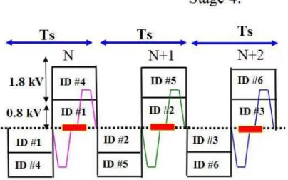
4.1 Pulse density control……….. 42
4.2 Staging……… 43
4.3 Intermittent operation and sorting……….. 44
5. Simulations……….. 46
6. Necessary device - long -pulse induction acceleration cell……… 54
6.1 The droop………... 54
6.2 A 2:1 transformer as a long-pulse induction acceleration cell…….. 55
6.3Characteristics of the 2-turn induction cell………... 56
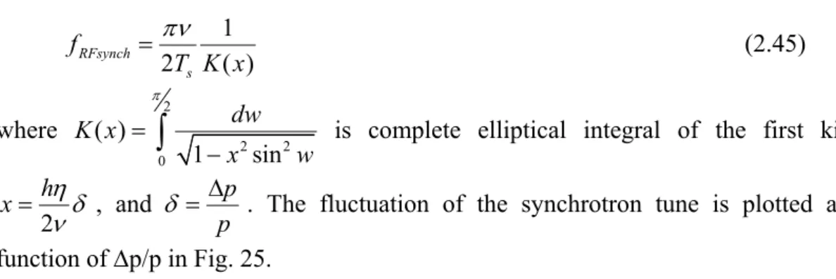
6.4 Voltage profile of the modified induction cell………. 58
6.5 Sequential and parallel operation of long-pulse induction cells…. 61 7. Beam Simulator ………. 62
8. Intelligent acceleration control system for the KEK-DA……… 65
8.1 Stage selector………. 66
8.2 DSP sets for generating dynamic pulse width and amplitude……… 67 8.3 Frequency dividers for intermittent operation ……….. 68
8.4 Logic units………. 70
8.5 Induction acceleration control system……… 70
9. Experimental results of the acceleration scheme using a beam simulator 76
10. Conclusion ……… 80
Appendix References List of figures
List of tables
Constants
Abstract
A novel ion accelerator referred to as a digital accelerator, which is based on the induction synchrotron concept, is discussed here. Its operational performance is the same as that of the induction synchrotron, where acceleration and confinement of ions in the propagation direction are implemented independently with a pulsed voltage and the so-called barrier voltages. These voltage pulses are generated in the induction acceleration cell energized by the switching power supply, which is triggered with a trigger signal manipulated by an ion-bunch signal. In the digital accelerator, any ion species with its possible charge state can be accelerated since the acceleration voltage pulse generation is always synchronized with the ion circulation. Acceleration of argon ions is planned as a proof-of-principle experiment at KEK. The detailed aspects of the digital accelerator are described, including theoretical backgrounds such as beam dynamics.
The KEK-PS booster synchrotron is under renovation, aiming to become the first digital accelerator. The KEK Booster is a rapid-cycle synchrotron where the acceleration voltage amplitude changes dynamically throughout the acceleration period. The existing induction cells can provide a peak output voltage of 2 kV in 250 nsec pulse width at a maximum repetition rate of 1 MHz. Once the peak output voltage is fixed, it is difficult to change its magnitude in the same acceleration cycle. The main purpose of this thesis is to propose the realization of a dynamically changeable acceleration voltage by employing the induction acceleration system. In fact, this idea has been developed for the KEK digital accelerator. The acceleration period is divided into stages, where different acceleration voltages, pulse widths, and repetition rates are required. A novel technique, which consists of staging of the acceleration period, systematic sorting of the induction acceleration cells, and intermittent operation of the induction acceleration systems, has been developed. Particle tracking simulations in the longitudinal direction were performed in order to verify the feasibility of the scheme. The acceleration scheme has been verified experimentally for the first two stages of the acceleration period by using a beam simulator signal. The results will be presented here and the perspectives of this technique will be discussed.
Chapter 1 Introduction
The KEK digital accelerator (KEK-DA) is based on the induction synchrotron (IS) concept [1], which was demonstrated in 2006 [2]. In the induction synchrotron concept, pulse voltages are used to accelerate and confine particles. Almost rectangular-shaped voltage pulses are obtained by 1-to-1 transformers referred to as induction cells, which are energized by individual switching power supplies. The switching power supplies are fired by triggering their solid-state switching elements with digitalized trigger signals, which are generated by the bunch monitor signal. Using the pulsed-power technology newly developed at KEK, these voltage pulses can be generated at frequency values ranging from extremely low to up to 1 MHz, and are synchronized with the circulation of the ion bunch. This property makes the KEK- DA a versatile accelerator which can accelerate any kinds of ions from a very low energy.
The KEK-DA is unique from the operational point of view as it is based on a digital technique referred to as pulse density control. Using pulse density control, fixed output voltages from the induction cells can be modulated over time to provide the required energy gain to the particles. This feature is developed extensively in the KEK-DA acceleration scheme.
The KEK-DA is a modification of the KEK-PS booster ring (BR). BR had been operated at 20 Hz over more than 30 years as a rapid-cycle synchrotron (RCS). The acceleration voltage in an RCS changes dynamically throughout the acceleration period. The output voltage of the induction acceleration system, which has been developed for the IS, is fixed because of the nature of the construction. The most serious issue concerns the implementation of dynamic changes in the required acceleration voltage by the induction acceleration system with a constant output voltage. In addition, the trigger frequency, which is synchronized with the revolution frequency, must be varied over more than two orders of magnitude. The revolution frequency during the acceleration exceeds the maximum switching frequency of the present induction acceleration system.
In order to meet the technical requirements for the acceleration system of the KEK- DA by assuming the existing induction acceleration system with a maximum operation frequency of 1 MHz and 2 kV constant output voltage, a novel and specific acceleration scenario has been explored, and necessary hardware has been developed. The present thesis covers all details related to the acceleration scenario in the KEK- DA and the actual induction acceleration system for the KEK-DA. The noteworthy properties in the developed induction acceleration technique can be summarized as follows.
(1) A pulse width is varied in accordance to the acceleration and
(2) The effective acceleration voltage is varied in accordance to the acceleration.
The acceleration scheme combining the 2 μsec pulse and shorter pulse voltages has been verified with the aid of computer simulation. Furthermore, the necessary long pulse induction cell was developed, and its performance was analyzed. An intelligent acceleration control system was developed for the purpose of maneuvering the long pulse induction cells and the existing short pulse induction cells. The control system was tested using a beam simulator signal as an alternative of the circulating beam, which was developed in order to verify this rather sophisticated acceleration system. The KEK-DA is a medium-energy synchrotron, and all kinds of ions, including cluster ions in any possible charge state and mass, can be accelerated in a single ring. Such an accelerator should be attractive for researchers in various fields. Irradiation of various ions on metals, magnetic materials, ceramics, semiconducting materials and polymers produces new materials such as nano-wires, nano-transistors, quantum dots and conducting carbon tracks within diamond insulators. Deep implantation of moderate-energy heavy ions can create alloys of bulk size. Warm dense matter science studies will greatly benefit from heavy-ion beams in exploring high-density and high-temperature regions where the equation of state is not yet explored. A cost- effective hybrid cancer therapy can be realized using a single DA, from which protons and carbon ions can be provided. Ion beam mutagenesis is also an attractive and necessary application where the DNA structure of plant seeds is altered to produce new species. We might be able to create new species of plants which can retain their productivity even in the conditions of significant climate changes in this century.
In this thesis, Chapter 1 introduces various particle accelerators, followed by detailed description of the induction synchrotron concept. Its key devices and the proof-of- principle experiment are described. In Chapter 2, the longitudinal dynamics is developed for both cases of RF and induction synchrotrons and transverse dynamics is briefly introduced. Chapter 3 discusses the outline of the KEK-DA. The newly developed acceleration scheme, which is developed for the KEK-DA, is described in detail in Chapter 4. The results of the simulations carried out in order to verify the feasibility of the acceleration scheme are discussed in Chapter 5. The induction acceleration cell for a long acceleration pulse, which is required for the KEK-DA, is described together with its parameters and output waveforms in Chapter 6. The description of the development of the beam simulator is given in Chapter 7, and Chapter 8 describes the details of an intelligent control system for the KEK-DA. Subsequently, the experimental results of the induction acceleration system using a beam simulator signal are given in Chapter 9, followed by the conclusion derived from the results presented in this thesis.
1.1 Particle Accelerators
Machines capable of accelerating charged particles with the help of electromagnetic fields are referred to as particle accelerators. The charged particles can be electrons, protons, heavy ions, radioactive ions or cluster ions. The history of particle accelerators dates back to the 1930’s when electrons were accelerated using DC voltage. Present-day particle accelerators have evolved considerably, currently being some of the most sophisticated devices using the latest technology. Particles accelerators can be divided into two main categories:
a. Linear accelerators and b. Circular accelerators.
In linear accelerators, charged particles travel in a straight path, while in circular accelerators the particle trajectory is circular. Normally, electric field is used for accelerating the particles, and magnetic field is used for bending the trajectory of the particles.
Accelerators are indispensable tools for learning about the sub-atomic and sub nuclear dimensions. Relativistic particle beams from accelerators are capable of resolving the internal structure of the nucleus and its constituent sub-nuclear particles, similarly to a microscope. This is possible since the de Broglie wavelength,λB of highly energetic particles is smaller than the size of the nucleus, which is ~10-15m.
P P
B
h h c
p E
λ = = (1.1)
where, hP is the Planck constant, p is the momentum, and E is the energy of the particle. The energy of the particles is expressed in terms of electron volts (eV), where 1 eV=1.602x10⁻¹⁹ J. This is defined as the energy gained by an electron as it crosses a potential difference of 1 V. keV (103), MeV (106), GeV (109) and TeV (1012) are also used as units for describing particles with higher energies.
In the past, many large-scale accelerators referred to as "colliders" were constructed for the purposes of particle physics studies in an attempt to understand and reveal the nature of the Universe. Colliders are accelerators in which a collision between two beams rotating in opposite directions is done, releasing very high energies. In this regard, KEKB in Japan collide electrons and positrons for the purpose of studying the CP violation. Tevatron in Fermilab is used to accelerate and collide protons and antiprotons. The scale of the energies handled in these machines can be fathomed by their sizes. The KEKB ring has a circumference of 3 km, and that of the main ring of Tevatron is 6.5 km. The upcoming Large Hadron Collider (LHC) at CERN, Geneva has a circumference of 27 km, and it will be utilized for accelerating protons in opposite directions. This accelerator will be used to search for the Higgs particle, as well as to study super symmetry and dark matter.
Today thousands of small accelerators exist which are used for a variety of applications, from radiotherapy for cancer treatment and material science studies to the treatment of biomedical waste, high energy physics studies and the treatment of radioactive waste among others.
A brief history of accelerator development over the years is provided below in order to understand the evolution of accelerators over time.
1.1.1. Electrostatic accelerators
The first particle accelerator was the electrostatic accelerator [3]. In an electrostatic accelerator, charges are accelerated by a ground potential to a very high potential produced by a high voltage generator, as shown in Fig. 1. The simplest example of an electrostatic accelerator is the electron gun of an ordinary TV set. Electrons flow from the cathode at ground potential towards the anode, which is kept at higher potential. The pioneering work in this field was done by Van de Graaff, and these accelerators are commonly referred to as Van de Graaff accelerators. Electrostatic accelerators can provide voltages of up to ~ 10 MV. This limit arises due to electrical breakdown. For voltages above 1 MV, pressurized gas is used to increase the breakdown limit of the high-voltage components. These accelerators are useful for low-energy applications with moderate beam currents. Normally, they act as injectors to upstream accelerators such as linear accelerators. Nowadays, tandem Van de Graaff accelerators are commonly used in which ions are accelerated from ground to high potential, after which the charge is stripped and accelerated again to ground potential, thus gaining double acceleration in the process. The main limitation of electrostatic accelerators is that the maximum achievable energy which can be obtained is directly proportional to the maximum voltage which can be applied without breakdown. RF accelerators are employed to overcome this limit.
Fig.1. A schematic diagram of the Van de Graaff accelerator
1.1.2. Linear accelerators
In order to overcome the limitations of corona formation and discharge on electrostatic accelerators, Ising (1924) proposed high frequency voltage, i.e. RF voltage. In RF devices, there is no buildup of voltage with respect to the ground. Such devices were first used as linear accelerators. As the name suggests, linear accelerator accelerate particles along a linear trajectory. An abbreviated form linac is commonly used for linear accelerators. Linacs followed electrostatic accelerators and were able to accelerate charged particles to energies above MeV. Earlier linear accelerator had many short accelerating sections, each applying RF voltage. For the proper acceleration of particles, the phase of RF is adjusted in order for particles to "see" rising voltages during the transit through the gap, hence gaining energy, while at other times the particles are shielded from the decelerating RF field by the drift tube. As the particle energy increases, its velocity also increases together with the distance between gaps. As the particle become relativistic, the gap becomes almost constant. This type of accelerator was first developed by Wideroe and later in a modified form by Alvarez [4]. Linacs of the Alvarez type are still used for proton and ion beam acceleration. Linac technology is currently highly developed, giving high voltage gradient per gap and thus becoming shorter in length. The main advantage of using linear accelerators is their capability to produce high energies and high-quality beams. The high-quality attributes are small energy spread and small beam size. In principle, linear accelerators have no limits. Acceleration units can be added indefinitely, thus achieving higher and higher energies. However, the cost of the structure increases as the length increase, which determines the effective limit. Examples of linac include the 40 MeV proton linac of KEK-Proton synchrotron (KEK-PS) shown in Fig. 2, the 2-mile long electron linear accelerator developed at Stanford for acceleration of electrons, and UNILAC at GSI in Germany for the acceleration of ions. The proposed International Linear Collider (ILC) backbone is a linear accelerator. In the proposed design, a 12 km long accelerator section will accelerate electrons to 500 GeV, and another 12 km section will be used for the acceleration of positrons using superconducting cavity technologies. Linac find application as electron-positron colliders for high energy physics experiments, high-quality electron beams for free- electron lasers, pulse neutron sources for material science studies, and X-ray sources for radiotherapy to name a few.
Fig. 2. The 40 MeV Proton linac of KEK-PS
1.1.3. Cyclotrons
Cyclotrons are in the category of circular accelerators. In a circular accelerator, particles are accelerated along a circular path. Magnetic fields are used to bend the trajectory of the particles, and electric fields are used to provide the acceleration. With the ever increasing demand for higher particle energies, the cost of particle accelerators becomes an important factor. Therefore, circular accelerators were developed where particles are injected into a circular orbit, gaining energy at each turn from the RF cavities. When magnetic field is applied in perpendicular direction to the motion of a charged particle, the particle trajectory becomes circular. This principle was used by E. O. Lawrence to accelerate particles in cyclotrons [5]. The governing principle can be simply written as
Mv2
ρ =qvB (1.2)
where M is the mass of the particle, v is the velocity, ρ is the bending radius, q=Ze is the charge of the particle, and B is the applied magnetic field. Rearranging Eq. (1.2), we can write
v qB M
= ρ (1.3)
The timeτ required for the completion of one revolution is written as
2 2 M
v Bq
πρ π
τ = = (1.4)
The angular frequency ω is written as qB
ω= M (1.5)
Thus, the period of revolution does not depend on the velocity or the size of the orbit, but only on the strength of the magnetic field and the charge to mass ratio, since M = ⋅ where A is atomic mass number and mA mp p is the proton mass. Therefore, if all quantities are fixed, then the oscillator can be tuned to a frequency which alters the polarity of the electrodes referred to as "dees", which are shown in Fig. 3. As the velocity increases, the radius of the path also increases and the particle reaches the dee radius, where it is extracted using extraction electrodes. In early cyclotrons, magnetic field decreased with the radius, putting a limit on the total energy which can be gained due to the increase of relativistic mass. The maximum energy which can be achieved with a cyclotron depends on q/A, where A is the atomic mass number. The limit on the cyclotron is determined by the size of the magnet. These accelerators provide a good balance between cost of the structure and energy of the particles. Hundreds of cyclotrons are used throughout the world for nuclear physics experiments, as well as for industrial and medical applications. The RIKEN superconducting cyclotron facility in Japan can accelerate ions ranging from a single proton to bismuth ions in a wide range of energies. Superconducting cyclotrons use high-field superconducting-magnet techniques with the basic isochronous cyclotron technology (magnetic field changes with the radius, thus causing the revolution frequency to remain constant). This high magnetic field reduces the cost and the size of the cyclotron.
Fig. 3. A schematic diagram of a cyclotron
1.1.4. Betatron
In the cyclotron, the magnetic field remains constant and the radius of the particle trajectory increases together with the applied energy. On the other hand, in betatrons the magnetic field is increased as the particle accelerates, and the radius of the orbit is thus maintained. The acceleration fields are due to the electromotive force generated by the varying magnetic field, and this effect is also known as Faraday’s law.
. .
S
E dl dB dS
= − dt
∫
G G∫
G G (1.6)The betatron makes use of the transformer principle where the secondary coil is replaced by the circulating beam in a closed doughnut-shaped vacuum chamber, as shown in Fig. 4. Betatrons were the first induction-based circular accelerators [6]. Transverse particle oscillation was first observed in a betatron, and the oscillation is now referred to as betatron motion for this reason. The magnetic fields in a betatron and the size of the magnet determine the upper limit on the maximum achievable energy. Most betatrons are used for accelerating electrons and producing hard X-rays for medical applications.
Fig. 4. A schematic diagram of a betatron.
1.1.5. Synchrotrons
Synchrotrons overcome the bulky magnet requirement posed by cyclotrons. For relativistic particles (v ≈ c), the bending radius, ρ increases together with the energy E=Mc2 according to the following equation
E
ρ = qcB (1.7)
Instead of allowing particles to spiral outwards as they gain energy, as in cyclotrons, the particles are made to rotate at a constant radius in a synchrotron. Therefore, for a constant radius, the ratio of E/B should be constant, which means that the magnetic field B must be increased synchronously with the energy [7]. The magnets for bending and focusing are arranged in such manner that the particles are confined to an almost circular orbit. This arrangement is referred to as lattice. The lattice can consist of magnets with combined function (the same magnets are used for both focusing and bending) or with separate function (separate magnets for focusing and bending). The magnetic field cannot be varied from 0 to the maximum level, and therefore the ions need to be injected into the synchrotron with some minimum energy. For this purpose, pre-acceleration injectors such as linac are used. Synchrotrons have straight sections for injection, extraction, RF cavities, vacuum stations, and auxiliary magnets. The acceleration voltage Vac is written as (Appendix A)
0 ac
V C dB ρ dt
= (1.8)
where C0 is the circumference, and the changing magnetic field, dB/dt needs to be controlled accurately for the proper acceleration of the particles. Usually, Vac is written as
ac rf sin s
V =V φ (1.9)
where Vrf is the RF voltage provided by the RF cavity, and φs is the phase of the ideal particle referred to as synchronous particle. The phase of the particle is controlled in real time to provide the design acceleration voltage to the particles. Thus, control becomes important in these machines, where it is usually provided by RF feedback systems.
To date, synchrotrons produce the highest energies, usually reaching TeV. KEK-PS, shown in Fig. 5, is a 12 GeV proton synchrotron, KEKB is an 8 GeV electron- positron collider, JPARC has a 3 GeV and a 50 GeV ring for protons, and LHC is a 7 TeV proton-proton collider.
Fig. 5. KEK-12 GeV proton synchrotron ring composition 1.2 Induction synchrotron
The concept of induction synchrotron (IS) was proposed by Takayama and Kishiro in 2000 for the purpose of overcoming the limits posed by RF acceleration [1].
In this concept, the acceleration and the confinement of the particles is achieved independently by using two transformers instead of the resonant cavity in the RF synchrotron. The almost rectangular-shaped voltage pulses are obtained by 1-to-1 transformers referred to as induction cells, which are energized by individual switching power supplies. The switching power supply is fired by triggering solid- state switching elements (power MOSFET) with trigger signals generated in a digital signal processor, DSP, where the bunch monitor signal is manipulated digitally. Consequently, the acceleration and the confinement are automatically synchronized with the beam revolution. The IS concept was demonstrated in its complete form in a proof-of-principle experiment in 2006 [2].The principle is shown in Fig. 6(a) together with that of the RF synchrotron.
Fig. 6(a). A Schematic diagram of the RF synchrotron and the induction synchrotron.
This characteristic feature allows us to accelerate any ions in any of their possible charge states from an extremely low energy to high energy in a single ring. Namely, an injector-free synchrotron can be realized as shown in Fig. 6(b).
Fig. 6(b) Accelerator configuration
The acceleration and the longitudinal confinement of the charged particles are independently carried out using induction pulse voltages, as shown in Fig. 7. A long- pulse voltage generated in the induction acceleration cells provides the acceleration voltage. A pair of pulse voltages with opposite signs, which is generated in other induction cells, is capable of providing longitudinal focusing forces. This property is rather effective for increasing the freedom of beam handling in longitudinal direction. By increasing the time duration between barrier voltages used for confinement, the longitudinal phase space, which is available for capturing ions, is effectively expanded to increase the average beam intensity while keeping the local line density below the transverse space-charge limit.
Fig. 7. Voltage profile of the induction synchrotron
The equivalent circuit diagram of the induction acceleration system is shown in Fig. 8. A DC power supply (DC-P.S.) energizes the switching power supply, and the high- voltage pulses are transferred to the induction cell via a 120 Ω transmission line. A matching resistance Z is connected in parallel to the induction cell to minimize reflections. R is the resistance representing the core loss. L is the inductance of the magnetic material, and C is the capacitance of the induction cell. In essence, the induction cell works as a 1:1 transformer, where the beam sees almost the same voltage as the one supplied by the DC P.S.
Fig. 8. Equivalent circuit for an induction acceleration system.
1.3 Key components of the induction synchrotron
The key components of the induction synchrotron are the induction cells, which provide pulse voltages, the switching power supply, which drives the cells, and a gate trigger control system, which fires the solid-state switching elements of the switching power supply. The following section will elaborate on these key components.
Induction cell
The induction cell is a key device in the induction acceleration system. The present induction cell was developed for the proof-of-principle experiment of the induction synchrotron using the KEK-PS, which was operated at a repetition rate of 667-882 kHz. The voltage induced through the induction cell is given by the following relation
max
ind P
V ⋅ = −τ B ⋅ ⋅ k S (1.10)
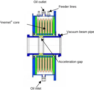
where Vind is the induced voltage, τP is the pulse length, Bmax is the maximum flux, k is the number of disks, and S= ⋅w d is the cross-section of the single disk-shaped magnetic material of thickness d and width w. The choice of magnetic material was very important due to high repetition rate, where a magnetic material with high permeability and low core loss was desired. Therefore, Finemet® FT-3M was used in the induction cell [8,9]. It is a nanocrystalline alloy with very high relative permeability, μ~104. The core loss depends on the excitation rate dB/dt and the flux swing ΔB. Therefore, core operation in a small B-H loop is desired. In the present design, ΔB is restricted to under 0.2 T. The magnetic core, being prone to corrosion, is cooled with silicon oil with a flow rate of 80 l/min. The oil is in turn cooled by water through a heat exchanger. The total heat load was estimated to be 18 kW. The cross- sectional view of the developed induction cell is shown in Fig. 9 [10]. Each induction cell consists of 6 Finemet® bobbins. The electrical parameters of the induction cell are given in Table 1. The maximum output voltage of the present induction cell is 2 kV. The induction acceleration cell is connected to the switching power supply by a 120 Ω transmission line. In order to ensure the proper matching with the transmission line impedance, a matching resistance of 210 Ω is connected in parallel to the induction cell.
Fig. 9. Cross-sectional view of the induction cell. Table 1. Electrical parameters of the induction cell
Capacitance (pF) 260 Inductance (μH) 110 Resistance (Ω) 330
Switching power supply
The switching power supply is a kind of power modulator [11], which is capable of generating bipolar rectangular-shaped voltage pulses at a maximum repetition rate of 1 MHz, as shown in Fig. 10. It consists of a DC power supply and a switching power supply. The switching power supply works as a full bridge circuit consisting of four identical switching arms, where each arm is composed of 7 power metal oxide semiconductor field effect transistors (MOS-FETs), MOS-FET DE475-102N21A by IXYSRF, connected in series. Each arm is capable of handling a maximum of 2 kV and 20 A. The MOS-FET gates are driven by their own gate driving circuits which are electrically isolated with extremely low capacitive DC-DC converters from their primary power source. The gate signals are generated by converting optical signals, which are provided from the pulse controller, into electronic signals. The maximum switching frequency is limited to 1 MHz due to heat deposition problems in the switching elements. The MOS-FET’s are attached to a copper heat sink which is cooled by water. The rating of the switching power supply, which was developed in collaboration between KEK and Nichicon Company, is given in Table 2 [12].
Table 2. Specifications of the switching power supply DC power supply (kW) 50 Output voltage (kV) 2.5 Peak output current (A) 20 Duty of pulse (%) 50 Power loss at switching element (W) 200
Oil inlet Oil outlet
Feeder lines
Acceleration gap Vacuum beam pipe Finemet® core
Fig. 10. Switching power supply
The DC Power supply (DC-PS) is used for energizing the switching power supply at a maximum rating of 2.5 kV at 20 A.
Fig. 11. DSK 6416 unit
The bunch signals are processed with a Texas instruments C6000 series 1 GHz DSP for generating the gate trigger signals for the switching power supply, which is shown in Fig. 11. A master signal for the gate trigger signal is first transferred to an optical trigger unit, which is shown in Fig. 12, and is then divided into the necessary number of signals which need to be sent through an optical fiber cable to individual switching elements in the gate driving circuit, thus maintaining the insulation from the high- voltage circuit.
Fig. 12. Optical trigger unit
The layout of the hardware components is shown in Fig. 13. The induction cells were installed in the main ring of the proton synchrotron. Gate trigger generation and observation was performed at the central control room (CCR). The DC power supply was placed inside the power supply building of the booster magnet, and the switching power supply was placed at a distance from the induction cell in the accelerator tunnel in order to avoid radiation exposure of the switching elements.
Fig. 13. Hardware components of the induction synchrotron.
1.4 Proof-of-principle (POP) experiment of the induction synchrotron
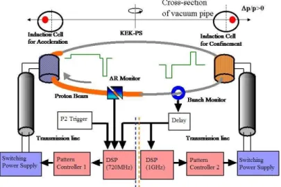
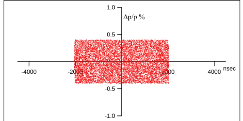
The induction acceleration experiment was carried out using the KEK 12 GeV proton synchrotron (12GeV-PS) in a series of proof-of-principle (POP) experiments in order to demonstrate the concept of the induction synchrotron. As the first step, the induction acceleration in a high-energy circular ring was demonstrated in 2004 [13], in which a single proton bunch injected from the 500 MeV booster ring and captured in an RF bucket was accelerated from 500 MeV to 8 GeV. This means that a hybrid synchrotron with functional separation in the longitudinal direction had been realized. As the second step, barrier bucket trapping was demonstrated where a proton bunch captured by the induction barrier voltages at an injection energy of 500 MeV survived for more than 450 msec [14]. In the experiment in the third and final step in 2006, particles were confined and accelerated by induction pulse voltages provided by induction cells. The gate signals used to turn on the MOS-FETs were generated in the gate control system by manipulating both signals—one monitored using the fast bunch monitor and the other using the beam position monitor—using a digital signal processor and active delay modules [15]. A schematic diagram of the control system is shown in Fig. 14. The machine and the induction cell parameters are given in Table 3. In this demonstration, the beam-orbit control was the most important issue, as in any other synchrotron. Without this function, charged particles are not efficiently accelerated in the vacuum chamber. The so-called ΔR-feedback system is equipped to meet this requirement similarly to a conventional RF synchrotron, where the RF phase seen by the bunch center is automatically adjusted in real time to compensate for any surplus or shortage of acceleration. A similar feedback system [15], where the gate pulse generation was determined by integrating the digital gate pulse generator with the orbit information proportional to the momentum error, Δp/p, was introduced in the IS. The beam position monitor directly gives ΔR=D(s)Δp/p, where D(s) is the momentum dispersion function at the location of the beam position monitor. When the signal amplitude exceeds a preset threshold value, the gate trigger signal is blocked in the DSP. Accordingly, the acceleration voltage pulse is not generated in the next turn, and the momentum of the bunch centroid approaches the correct value, which is uniquely determined by the bending field. Throughout the acceleration process, the central orbit of the bunch was kept at a constant value, as expected.
Fig. 14. A schematic diagram of an induction synchrotron control system used in the POP experiment.
The results of the proof-of-principle experiment are shown in Fig. 15. The KEK PS is essentially a slow cycling synchrotron. It was operated at a repetition rate of 0.25 Hz for this experiment. Its operational pattern in the present experiment is composed of a constant minimal field period of about 450 msec and an acceleration period of 2.2 sec for the 6 GeV acceleration pattern. A single proton bunch with an energy of 500 MeV was injected from the booster ring into the main ring and was accelerated to an energy of 6 GeV, which was determined by the ramping pattern of the bending magnet. The first waveform is the ΔR signal, which shows the orbit of the beam throughout the acceleration process. The slow intensity monitor signal (yellow) shows some beam loss at the beginning and 400 msec after the onset of the acceleration. Furthermore, the acceleration voltage pulse is shown in pink, the bunch monitor signal is shown in blue, and the magnet ramping profile is shown in orange.
Fig. 15. Results from the proof-of-principle experiment of the induction synchrotron. From top to bottom, ΔR feedback signal (green), slow intensity monitor signal
(yellow), acceleration voltage pulses (pink), bunch monitor signal (blue), and bending magnet ramping pattern (orange).
Table 3. Machine and induction cell parameters for the POP experiment Machine parameter Value
Injection energy (MeV) 500 Transition gamma, gt 6.63
Circumference, C0 (m) 339.48 Bending radius, ρ (m) 24.4
Induction parameter Value Acceleration voltage (kV) 6.4 Barrier voltage (kV) 10.8
Chapter 2 Longitudinal and transverse beam dynamics
In contrast to the RF synchrotron, the functions of acceleration and confinement of particles are separated in the induction synchrotron, as shown in Fig. 7. The longitudinal motion in the case of RF and induction synchrotrons is given in detail in order to distinguish the features in each case [16]. Understanding the concept of longitudinal motion in the induction synchrotron is required for controlling the barrier voltage parameters for the proper confinement of the particles. A detailed derivation of the synchrotron motion in the induction synchrotron is given. The analytical results are verified with the experimental results, obtained during the proof-of-principle experiment for the induction synchrotron, by using computer simulations. The software was then used for longitudinal particle acceleration simulations for the KEK- DA. Transverse motion remains the same for ions (Appendix B).
2.1 Longitudinal dynamics of RF synchrotrons
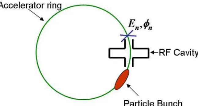
In the case of RF synchrotrons, energy and phase equations can be written in a discrete form assuming that RF devices are placed at a certain position in the accelerator ring shown in Fig. 16. The synchronous particle is always accelerated with the designed acceleration voltage V, which is uniquely determined by the magnetic ramping pattern of the accelerator given by Eq. (1.8). Its dynamical variable is denoted by a subscript‘s’. The schematic of RF voltage and the bunch position is shown in Fig. 17. Two dynamical variables, the energy E and the phase φ, are used for developing the model. The former is the total energy of a particle and the latter is defined byωst, where ωsis the angular frequency of the ideal particle (synchronous particle), and t is the time. These dynamical variables are measured immediately before entering the RF acceleration device. The total energy E gained by a synchronous particle after (n+1)th turn is given by Eq. (2.1).
Fig. 16. A schematic diagram of the accelerator ring showing an observation point.
1 sin
s s
n n s
E + =E +ZeV φ (2.1)
where Ens+1 is the energy of the synchronous particle at the (n+1)th turn
s
E is the energy of the synchronous particle at the nn th turn φs is the synchronous phase
V is the acceleration voltage as seen by the synchronous particle e is the unit charge
Z is the charge state of the particle
The energy of an arbitrary particle after (n+1)th turn is given by
1 sin
n n
E + =E +ZeV φ (2.2)
where En+1 is the energy of the synchronous particle at the (n+1)th turn E is the energy of the synchronous particle at the nn th turn φ is the phase of an arbitrary particle
Fig. 17. RF acceleration voltage and synchronous particle phase.
The Difference in energy between an arbitrary particle and the synchronous particle at the (n+1)th turn is written as
1 (sin sin )
n n s
E + E ZeV φ φ
Δ = Δ + − (2.3)
Similarly, the difference in phase between an arbitrary particle and the synchronous particle is written as
1
1
n n 2
n
h p φ + φ η π p
+
⎛Δ ⎞
Δ = Δ + ⎜ ⎟
⎝ ⎠ (2.4)
where
1 +1
+ ⎟⎟⎠
⎜⎜⎝ ⎞
= ⎛ Δ
⎟⎠
⎜ ⎞
⎝
⎛ Δ
n p n
η p
ττ (2.5)
ωrf =h ωs is the angular frequency of the RF voltage h is the harmonic number
p is the momentum
τ is the time to complete one revolution is the slippage factor, 12 12
t s
η=γ −γ (2.6)
γt is the transition gamma, and γs is the relativistic gamma for the synchronous particle.
Changing from the turn variable ‘n’ to the time variable ‘t’, it is assumed that the energy increments and accordingly the time period increments are small in comparison to the overall time changes, and therefore can be taken as constant over a
small time interval. Introducing a new variableW = ΔE ωs and taking the average of Eq.(2.3) over a revolution time period of 2π ωs, we have
1 (sin sin )
2 s
dW ZeV
dt = π φ− φ (2.7)
and
2
2 s
s s
d h
dt E W φ η ω
= β (2.8)
Equations (2.7) and (2.8) are equations of motion in (W, )φ space. Since the parameters change slowly with respect to time, we can assume the Hamiltonian to be independent of time, thus obtaining
( )
, 2 2 s2 2 2(
cos cos s ( s) sin s)
s s
h ZeV
H W W
E
φ = η ωβ + π φ− φ + −φ φ φ (2.9)
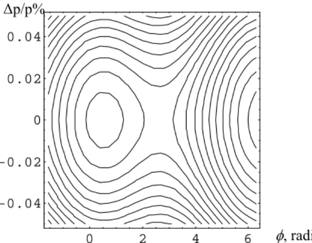
The Hamiltonian contour plot below the transition energy is shown in Fig. 18. The particles which lie inside the separatrix are stable, and particles which lie outside the separatrix are neither bound nor accelerated. The area of the separatrix decreases as the synchronous phase increases for the same RF voltage. Therefore, the number of particles which can be accelerated are limited in the case of RF synchrotron.
0 2 4 6
-0.04 -0.02 0 0.02 0.04
Fig. 18. Hamiltonian contours in phase space for the RF voltage For small amplitude phase oscillations, i.e. Δ = − << , we can write φ φ φs 1
(
sinφ
−sinφ
s)
=sin(Δ +φ φ
s) sin−φ
s ≈ Δφ
cosφ
s (2.10)Therefore, Eq. (2.7) can be written as 2 cos s dW ZeV
dt = π φ φΔ (2.11)
( )
2 2 2
2 2 2 cos
2
s s
s
s s s s
d h dW h ZeV
dt E dt E
φ η ω η ω φ φ
β β π
Δ = = Δ (2.12)
( ) ( )
2
2
2 s 0
d dt
φ φ
Δ + Ω Δ = (2.13)
The synchrotron frequency Ωs is given by
Δp/p%
φ, radians
2
2
cos 2
s s
s
s s
ZeVh E ω η φ
Ω = πβ (2.14)
For stable particle motion, the synchrotron frequency must be real. As η is negative below the transition energy, the synchronous phase is set to be in the range 0
s 2 φ π
< < . Above the transition energy, ηis positive, and therefore the synchronous phase is set in the range
2 s
π φ π< < . At the transition energy, the synchrotron motion freezes, and there is no phase focusing.
2.2 Longitudinal dynamics of the induction synchrotron
The induction acceleration cells in the KEK induction synchrotron are localized at several places. For the sake of simplicity, these cells, including the induction cells used for confinement, are represented as a single device in the present acceleration model. Ignoring the transit time through the acceleration device, the changes in E and φ per turn can be given by
( )
ΔE n+1= Δ( )
E n +Ze V{
( )φn −Vac}
(2.15)( )
1 2 1
2
n n n
s s
h E
E
φ + = +φ βπη Δ + (2.16)
where Δ = − ,E E Es V
( )
φn is the induction voltage as seen by the accelerated particle, as shown later, ηis defined as above, and γs and βsare relativistic gamma and beta, respectively. Introducing W = ΔE ωsas defined earlier, and taking the average over a revolution time period of 2π ωs, we have{
( )}
2
n ac
Ze V V
dW dt
φπ −
= (2.17)
2
2 s
s s
d h
dt E W φ η ω
= β (2.18)
These canonical equations are derived from the following Hamiltonian:
(
,)
2 2 s2 2 2{ ( )
ac}
s s
h Ze
H W W V V d
E η ω φ
φ = β − π
∫
φ′ − φ′. (2.19) As V( )
φn =Vbb +Vac, the integrand in Eq. (2.19) is simplified. It is reasonable to regard the Hamiltonian as a constant for a short time period, during which the changes in ,η βs, and E are rather small. A typical contour for the Hamiltonian is shown in s Fig. 19.Fig. 19. A schematic diagram of the Hamiltonian contours in an induction synchrotron. The bucket height in the case of the induction synchrotron can be calculated from the Hamiltonian given in Eq. (2.19). If ( )V φ′ =Vbb( )φ − , then the Hamiltonian reduces Vac to
2 2
( , ; ) 2 ( )
2 2
s
bb
s s
H W t W Ze V d
E φ
φ ω ηβ π φ φ
′
′ ′
= −
∫
(2.20)For the rectangular barrier voltage profile shown in Fig. 20, where the barrier amplitude isV ,bb φpulse =ω τs pulse and τpulseis equal to the flat top time, the integration of
( )
V φ′ gives Vbbτ ωpulse s. No rise time and fall time is assumed. Therefore, we can write
2 2
( , ; ) 2
2 2
s bb pulse s
s s
H W t W Ze V
E ω η ω τ
φ = β − π (2.21)
Fig. 20. Voltage profile of the rectangular barrier
In order to calculate the barrier height, we determine the maximum W at φ = , 0
2 2
max 2 max
( , 0;0) 0
2 2
s bb pulse s
s s
H W W Ze V
E ω η ω τ
β π
= − = (2.22)
This gives
nsec Arbitrary
units
2 2
max 2
2
s s s bb pulse
s
E Ze V
W β ω τ
ω η π
= (2.23)
or, in terms of p p
⎛Δ ⎞
⎜ ⎟
⎝ ⎠, where
2
s s
p E
p β E
Δ = Δ (2.24)
we obtain
2 max
bb pulse s
s s
p ZeV
p E
β ηπτ ω
⎛Δ ⎞ =
⎜ ⎟
⎝ ⎠ (2.25)
The barrier bucket height is thus proportional to the square root of the product of the barrier voltage and its pulse length in the induction synchrotron.
2.3 Synchrotron motion in the induction synchrotron
In order to calculate exactly the synchrotron frequency in the induction synchrotron, we start with a trapezoidal profile (more realistic with finite rise and fall times) of the barrier voltages V , as depicted in Fig. 21(a). In Fig. 21(b), the outer edges on the bb phase axis represent the oscillation amplitude of the particle. The motion in the barrier bucket is quantitatively divided into three regions: (1) drift in the null voltage region, (2) focusing in the parabolic potential, and (3) focusing in the linear potential. It should be noted that the motion in region (2) and (3) is subjected to adiabatic damping, as well as that the exact solution throughout the region is known for the abovementioned short time period.
Fig. 21. (a) Barrier voltage shape with three distinct regions encountered by the particles (b) A schematic diagram of the Hamiltonian contour in phase space (W,φ). In order to analyze the temporal evolution of this oscillation amplitude associated with the acceleration, we start from the canonical Eqs. (2.17) and (2.18). Differentiating Eq. (2.18) with respect to time and substituting Eq. (2.17) into the result, we obtain the second-order differential equation,
( )
2
2
( ) ( )
( ) 2 0
dA dt bb
d d ZeV A t
dt A t dt
φ φ φ
− + π = (2.26)
where the abbreviation, A t( )=hη ω βs2 s2Es is used. The temporal change in the phases of individual particles is governed by Eq. (2.26). Since the parameters in this equation include all the information associated with the acceleration, its solution can provide the motion in phase space throughout the acceleration period. In order to eliminate the damping term, a new variable, ( )u t =φ( ) / ( )t v t is introduced. Whenv t( )= A t( ), Eq. (2.26) reduces to
( )
22 2 2
2 2
3 ( ) ( ) 0
2 ( ) 4 ( )
dA dt d u d A dt
u t B t
dt A t A t
⎧ ⎫
⎪ ⎪
+⎨ − ⎬ + =
⎪ ⎪
⎩ ⎭ (2.27)
whereB t( )=ZeVbb( )φ A t( ) 2π . Since ( )A t is a slowly varying function of time, its first-order and second-order derivatives with respect to time are small. Accordingly, the second term in the left-hand side of Eq. (2.27) can be ignored in the following derivation. We arrive at a final form of the phase oscillation equation which must be solved,
2
2 ( )
d u B t
dt = − (2.28)
The restoring forceB t can be assumed to be constant during a single synchrotron ( ) oscillation period T , which is much shorter than(dA dt/ ) A . In addition, the synchrotron oscillation is symmetric in phase space, as depicted in Fig. 21 (b). If we obtain the exact solutions in regions I, II, and III as shown in Fig. 21 (a), the synchrotron frequency Ω =s 2 /π T can be written in an analytic form. The instantaneous amplitude of the phase, φ is written using the WKB approximation as
s
C A φ =
Ω (2.29)
where, C is a constant coefficient determined from the initial conditions.
Analytical solution for a trapezoidal barrier
Since all parameters are assumed to be constant throughout a single synchrotron oscillation period, the solution of Eq. (2.28) can be written analytically. In region I, it is written as
2 0 2
1 1
1 ( )
( ) ( )
2 4
I
ZeV A t
u t B t t c t c
= + = π + (2.30)
where c is calculated from the initial condition, and 1 V is the amplitude of the barrier 0 voltage pulse. In region II, Eq. (2.28) is described by
2
2
2 ( )
II
II
d u a
A t k u
dt v
⎛ ⎞
= − ⋅ ⋅⎜ + ⎟
⎝ ⎠ (2.31)
Introducing k =ZeV0 2πa1, where a1= Δ and ωs t1 Δ is the length of linear region of t1 the barrier voltage, we obtain a2 = Δ . The solution of Eq. (2.31) is well known, ωs t2 and is written as
( )
{ }
2 2
( ) sin ( ) 1 II
c a
u t kA t t t
v δ v
= − + − (2.32)
where c ,2 δ and t are constants which are determined from appropriate boundary 1 conditions. Using these analytical solutions, the respective time periods of the motions in regions I and II are evaluated as
( )
{
1 2}
1
0
4
( )
a a
t ZeV A t
π φ − +
= (2.33)
1 1
2 1
2
sin1
( ) t t a
kA t c
− ⎛ ⎞
= + ⎜ ⎟
⎝ ⎠ (2.34)
In region III, which is a drift region, the time period is straightforwardly written as
2 2 ( )
a c kA t , where a2 = Δ and ωs t2 Δ is the drift length of the barrier voltage pulse. t2 Thus, the time period to complete one quarter of an oscillation cycle, which is denoted with t , is given by 3
( )
{
1 2}
1 1 23
0 2 2
4 1
( ) ( )sin ( )
a a a a
t ZeV A t kA t c c kA t
π φ − + − ⎛ ⎞
= + ⎜ ⎟+
⎝ ⎠ (2.35)
The synchrotron oscillation period T =2π Ω =s 4t3 leads to
23
s t
Ω = π (2.36)
Here, we note that the synchrotron frequency depends on both the rise time and the drift length of the barrier voltage pulse. We can use these parameters to control the bunch length as desired.
Analytical solution when the bunch edge lies within the linear region
Fig. 22.(a) A schematic diagram of the rise-and-fall shape of the barrier pulse. (b) A Hamiltonian contour in phase space (W, φ).