Multi-group profile analysis for high-dimensional elliptical populations

Multi-group profile analysis for high-dimensional elliptical populations

Masashi Hyodo^†

†Department of Mathematical Sciences, Graduate School of Engineering, Osaka prefecture university, 1-1, Gakuen-cho, Naka-ku, Sakai-shi, Osaka 599-8531, Japan. E-Mail: [email protected].

Abstract

In this article, we deal with tests for the parallelism and flatness hypotheses in multi-group profile analysis for high- dimensional data. We extend procedures from the results for normal populations proposed by Harrar and Kong [S.

W. Harrar, X. Kong, High-dimensional multivariate repeated measures analysis with unequal covariance matrices, J.

Multivariate Anal. 145 (2016) 1–21] to results for elliptical populations. Specifically, for an elliptical population, we demonstrate the asymptotic normality of the statistics used in their study, and we propose a new approximate test by improving an estimator of the asymptotic variance. Using asymptotic normality, we show that the asymptotic size of the proposed test is equal to the nominal significance level, and we also derive the asymptotic power. Finally, we present simulation results and find that our results are superior to those found using the existing procedure.

AMS 2000 subject classification: Primary 62H15; secondary 62F05.

Key words: Profile analysis, statistical hypothesis testing, high dimension, elliptical population.

1. Introduction

We consider the multi-sample test problem for profile analysis for elliptical populations. Forg ∈ {1, . . . ,a}, let µg =(µg1, . . . , µgp)^⊤be a p-dimensional real vector,Λg ap×pnonnegative definite matrix andξg(·) a nonnegative function. Thep-dimensional random vectorXgis said to have an elliptically contoured distribution if the characteristic function ofXgcan be written as

ϕg(t)=eⁱt^⊤µgξg(t^⊤Λgt).

This will be denoted byXg ∼ Cp(ξg,µg,Λg). Note that the expectation and covariance matrix ofXg are E(Xg)=µg

and var(Xg)=−2ξg^′(0)Λg := Σg, respectively. Elliptical distributions include several special cases, for instance, the multivariate normal, multivariatet, and contaminated normal distributions referred to by Muirhead [9].

Let Xgi be ng independent and identically distributed (i.i.d.) copies of Xg for i ∈ {1, . . . ,ng}. We consider a procedure for testing the parallelism hypothesis

H01 :µg−µa=γg1pfor anyg∈ {1, . . . ,a−1} vs. A01 : notH01. (1.1) Here, γg is a unknown real constant and 1p = (1, . . . ,1)^⊤. We also consider a procedure for testing the flatness hypothesis

H02 :µg1=· · ·=µgpfor anyg∈ {1, . . . ,a−1} vs. A02 : notH02, (1.2) and the level hypothesis

H03 :γ1=· · ·=γa−1=0 vs. A03 : notH03. (1.3) Harrar and Kong [4] showed other expressions that are equivalent to hypotheses (1.1)-(1.3). Expression (1.1) is equivalent to

He01:µ^⊤K01µ=0 vs. Ae01:µ^⊤K01µ>0

with

K₀₁ =P_a⊗P_p,

whereµ=(µ^⊤₁, . . . ,µ^⊤a)^⊤ andPk=Ik−k⁻¹1k1^⊤_k fork∈ {a,p}. Other expressions equivalent to hypotheses (1.2) and (1.3) are also obtained:

He0x:µ^⊤K0xµ=0 vs. Ae0x:µ^⊤K0xµ>0 forx∈ {2,3}with

K02 =(a⁻¹1a1^⊤_a)⊗Pp and K03=Da⊗(p⁻¹1p1^⊤_p), whereD_a=diag(n₁, . . . ,n_a)−n⁻_(a)¹nn^⊤. Here,n=(n₁, . . . ,n_a)^⊤andn_(a) =∑a

g=1n_g.

Srivastava [12] derived the likelihood ratio test for hypotheses (1.1), (1.2), and (1.3) for two normal populations.

However, the likelihood ratio test for (1.1) and (1.2) cannot be applied to data sets, such as microarray data, for n(a)≪p, even for normal populations with covariance homogeneity.

In profile analysis, Takahashi and Shutoh [13] considered approximation tests for hypotheses (1.1) and (1.2) for two normal populations with equal covariance matrices. Harrar and Kong [4] extended these tests for multi- group normal populations without assuming equal covariance matrices. They also obtained the approximation test for hypothesis (1.3) based on matching moments.

On the other hand, some previous studies of profile analysis have investigated the effects of non-normality in pro- file analysis. Okamoto et al. [10] used a perturbation method to obtain the asymptotic expansions of the distributions of test statistics for elliptical populations. Maruyama [7] extended the results under more general conditions using a different method introduced by Kano [6]. Note that these results are derived for a large asymptoticn(a).

In this paper, we propose new approximation tests for (1.1) and (1.2) for high-dimensional elliptical populations without assuming equal covariance matrices. We note that the rank ofK₀₃ is at mosta−1. That is, it does not grow with pand hence, it does not make sense to consider a large asymptotic (n_(a),p). Thus, our primary interest is to test (1.1) and (1.2). To propose these approximation tests, for high-dimensional elliptical populations, we show the asymptotic normality of the test statistics proposed by Harrar and Kong [4]. As a result, asymptotic normality is also established for a high-dimensional elliptical population, but that is not a trivial result. Furthermore, improving the estimator of the asymptotic variance of these test statistics enables us to propose a new approximate test for (1.1) and (1.2) for a high-dimensional elliptical population.

The remainder of this paper is organized as follows. The preliminary results for approximation tests are presented in Section 2. Using the asymptotic results in Section 2, we construct approximate tests for (1.1) and (1.2) and derive the asymptotic sizes and powers of these tests for elliptical populations in Section 3. In Section 4, the numerical accuracy of the proposed tests is investigated. The application of the results is illustrated with a real data example in Section 5.

2. Preliminary asymptotic results We define a non-randoma×amatrix

(Ra)i j =

diifi= j ψδiδjifi, j.

withd_i, δi, ψ∈Rfori∈ {1, . . . ,a}. Then we consider following random variable:

T =X^⊤(Ra⊗Pp)X−

∑a g=1

d_gtr(P_pS_g) ng , where

X=(X^⊤₁, . . . ,X^⊤_a)^⊤, Sg= 1 ng−1

ng

∑

i=1

(Xgi−Xg)(Xgi−Xg)^⊤. Here,Xg =n⁻_g¹∑ng

i=1Xgi.

2

Remark 2.1. If ψ = −1, d_i = 1−1/a, andδi = 1/√

a for i ∈ {1, . . . ,a}, then T is the test statistic for H01. If ψ=d_i=a⁻¹,δi=1then T is the test statistic forH02.

Here,Tis an unbiased estimator ofµ^⊤(Ra⊗Pp)µ, i.e.,

E(T)=µ^⊤(Ra⊗Pp)µ. (2.1)

In addition, the variance ofTis obtained as follows:

σ²=

∑a g=1

2d²_gtr{(PpΣg)²} ng(ng−1) +

∑a g=2

g−1

∑

h=1

4ψ²δ²gδ²_htr(PpΣgPpΣh) ngnh

+4µ^⊤(R_a⊗P_p)



∑a g=1

1 ng

(ege^⊤_g)⊗Σg



(R_a⊗P_p)µ, (2.2) whereeidenotesi-th basis vector.

Remark 2.2. If Rais an idempotent matrix, then Ra⊗Pp is also an idempotent matrix, andµ^⊤(Ra ⊗Pp)µ = 0is equivalent to(Ra⊗Pp)µ=0. Thus, if Rais an idempotent matrix andµ^⊤(Ra⊗Pp)µ=0, then

E(T) = 0,

σ² =

∑a g=1

2d_g²tr{(PpΣg)²} ng(ng−1) +

∑a g=2

g−1

∑

h=1

4ψ²δ²gδ²_htr(PpΣgPpΣh) ngnh .

We investigate the asymptotic distribution ofT for elliptical populations. Our primary objective in this section is to derive the asymptotic distribution ofT under some assumptions.

Letngforg∈ {1, . . . ,a}be function ofp, i.e.,ng =ng(p), and

tr{(PpΣgPpΣh)ⁱ}for anyg,h∈ {1, . . .a}, i∈ {1,2} be function ofp. Then we assume following conditions:

(A1) lim_p→∞n_g(p)=∞, 0<lim_p→∞ⁿ_n^g(p)

h(p) <∞for anyg,h∈ {1, . . .a}, (A2) κg<∞for anyg∈ {1, . . .a},

(A3) tr{(PpΣgPpΣh)²}

{tr(P_pΣgP_pΣh)}² =o(1) for anyg,h∈ {1, . . .a}, where

κg=E[{(Xg−µg)^⊤Σ⁻g¹(Xg−µg)}²] p(p+2) −1. The parameterκgis called a kurtosis parameter.

To discuss examples satisfying the assumptions (A2) and (A3), we consider the following three density function ofZ= Σ⁻g^1/2(Xg−µg).

a) The multivariate normal distribution with density function f(z)= 1

(2π)^p/2exp (

−z^⊤z 2

) .

b) Theϵ-contaminated normal distribution with density function f(z)= 1−ϵ

(2π)^p/2 exp (

−z^⊤z 2

) + ϵ

(2πη²)^p/2exp (

−z^⊤z 2η² )

, (2.3)

forε∈[0,1] andη∈(0,∞).

c) The multivariatetdistribution withkdegrees of freedom with the density function f(z)= Γ[(k+p)/2]

Γ[k/2](kπ)^p/2 (

1+ z^⊤z k

)₋(k+p)/2

fork∈N. Here,Γ[·] denotes gamma function.

These distributions satisfy assumption (A2). Actually, the kurtosis parameter of a) is 0, the kurtosis parameter of b) is 1+ϵ(η⁴−1)

{1+ϵ(η²−1)}² −1,

and the kurtosis parameter of c) is 2/(k−4) fork >4. Examples of covariance matrices that satisfy (A3) are those with compound symmetry. Actually, ifΣg =(1−ρg)Ip+ρg(1p1^⊤_p), forg ∈ {1, . . . ,a}andρg ∈(−1/(p−1),1), then tr{(PpΣgPpΣh)²}/{tr(PpΣgPpΣh)}²=1/(p−1).

The following lemma provides the asymptotic normality ofTunder assumptions (A1), (A2), and (A3). The lemma assures us that the asymptotic normality of the statisticTis maintained for an elliptical population.

Lemma 2.1. Under assumptions (A1), (A2), and (A3), T −µ^⊤(R_a⊗P_p)µ

σ ⇝N(0,1)as p→ ∞.

Proof. See, Appendix A.2.

3. Principal results 3.1. Proposed test

In this subsection, we propose approximation tests using a normal approximation based on Lemma 2.1. The test statistics for (1.1) and (1.2) are given by

T₀₁ = X^⊤K₀₁X−

∑a g=1

( 1−1

a

)tr(PpSg) ng

,

T₀₂ = X^⊤K₀₂X−

∑a g=1

tr(P_pS_g) ang

,

respectively. These statistics are also used in Harrar and Kong [4]. From (2.1), (2.2), and Remark 2.2, their expectation and variance for elliptical populations are summarized by the following equations. Forx∈ {1,2},

E(T0x) = 

0 under H0x,

µ^⊤K_0xµ(>0) under A0x. var(T0x) = 

σ²_H0x under H0x, σ²_A0x under A0x. Here, forx∈ {1,2}with

σ²_A0x =σ²_H0x+4µ^⊤K_0x



∑a g=1

1 ng

(ege^⊤_g)⊗Σg



K_0xµ, 4

where

σ²_H01 =

∑a g=1

( 1−1

a

)2 2tr{(P_pΣg)²} ng(ng−1) +

∑a g=2

g−1

∑

h=1

4tr(P_pΣgP_pΣh) a²ngnh , σ²_H02 =

∑a g=1

2tr{(PpΣg)²} a²n_g(n_g−1) +

∑a g=2

g−1

∑

h=1

4tr(PpΣgPpΣh) a²n_gn_h .

In practical use, it is necessary to estimate the asymptotic varianceσ²_H0x. Harrar and Kong [4] used the following estimator:

tr{(P^pΣg)²} = (ng−1)² (ng+1)(ng−2)

[

tr{(PpSg)²} −{tr(PpSg)}² ng−1

]

, (3.1)

tr(P\pΣgPpΣh) = tr(PpSgPpSh). (3.2)

Under elliptical populations, the expectations of them are calculated as following:

E[tr{(P^_pΣg)²}] = tr{(P_pΣg)²}+κg(n_g−1)

ng(ng+1)[{tr(P_pΣg)}²+2tr{(P_pΣg)²}], E{tr(P\_pΣgP_pΣh)} = tr(P_pΣgP_pΣh).

Thus, the estimator (3.1) has a bias for elliptical populations except whenκg =0.

We use the same estimator of tr(P_pΣgP_pΣh) as Harrar and Kong [4], but different estimators of tr{(P_pΣg)²}, which is defined as follows:

tr{(P\pΣg)²} = ng−1 n_g(n_g−2)(n_g−3)

[(ng−1)(ng−2)tr{(PpSg)²}+{tr(PpSg)}²−ngMg

], (3.3)

where

Mg= 1 n_g−1

n_g

∑

i=1

{(Xgi−Xg)^⊤Pp(Xgi−Xg)}².

Some properties of the estimators (3.2) and (3.3) are summarized in the following lemma.

Lemma 3.1. The estimatorstr{(P\pΣg)²}andtr(P\pΣgPpΣh)are unbiased, and rate consistent estimator, i.e. under (A1) and (A2),

tr{(P\pΣg)²}

tr{(P_pΣg)²} =1+op(1), tr(P\pΣgPpΣh)

tr(PpΣgPpΣh) =1+op(1) asp→ ∞.

Proof. See, Appendix A.3.

Remark 3.1. If Ppis replaced by Ip,tr(P\pΣg)²is the same as that of Himeno and Yamada [5].

Using (3.2) and (3.3) yields b σ²_H01 =

∑a g=1

( 1−1

a )2

2tr{(P\pΣg)²} n_g(n_g−1) +

∑a g=2

g−1

∑

h=1

4tr(P\pΣgPpΣh) a²ngnh

,

b σ²_H02 =

∑a g=1

2tr{(P\pΣg)²} a²n_g(n_g−1) +

∑a g=2

g−1

∑

h=1

4tr(P\pΣgPpΣh) a²n_gn_h ,

as the unbiased estimators ofσ²_H

01 andσ²_H

02, respectively.

Since

√bσ²_H0x/σH0x =1+op(1) asp→ ∞under (A1) and (A2), Lemma 2.1 and Slutsky’s theorem complete the following null asymptotic normality. Forx∈ {1,2}, under (A1), (A2), (A3), andH0x,

T0x

√bσ²_H0x ⇝N(0,1) (3.4)

asp→ ∞.

Based on the asymptotic normality (3.4), we propose the following approximation tests:

rejectingH01⇐⇒T01≥ √ b

σ²_H01z_α, (3.5)

rejectingH02⇐⇒T02≥ √ b

σ²_H02z_α, (3.6)

wherez_αdenotes upper 100αpercentile of standard normal distribution.

3.2. Asymptotic size and power

In this subsection, we investigate sizes and powers of test (3.5) and (3.6).

First, we investigate the asymptotic sizes of tests (3.5) and (3.6). Using (3.4), forx∈ {1,2}, under (A1), (A2), and (A3) yields

Pr (

T0x≥ √ b

σ²_H0xz_α|H0x

)=α+o(1)

asp→ ∞.

Next, we investigate the asymptotic powers of tests (3.5) and (3.6). Using if Lemma 2.1 and Lemma 3.1, we have the following theorem summarizing the asymptotic powers of tests (3.5) and (3.6).

Theorem 3.1. For x∈ {1,2}, under (A1), (A2), and (A3), Pr

(

T0x≥ √ b

σ²_H0xz_α|A0x

)= Φ

(µ^⊤K0xµ σ_A0x

−σ_H0x

σ_A0x

z_α )

+o(1)

as p→ ∞, whereΦ(·)denotes the cumulative distribution function (CDF) of the standard normal distribution.

Proof. See, Appendix A.4.

Thus, if the difference betweenH0xandA0xis not too small in thatµ^⊤K0xµis of the same order asσ_A0x or of a higher order, the test will be powerful. Conversely, if the difference betweenH0xandA0xis so small thatµ^⊤K0xµis of a lower order thanσ_A0x, the test will not be powerful and cannot distinguishH0xfromA0x.

4. Simulation and real example 4.1. Simulation

In this section, we perform Monte Carlo simulation for some selected parameters in order to verify the superiority of our test as compared to Harrar and Kong’s tests for (1.1) and (1.2) when the kurtosis parameter is not 0.

In our simulation, we compare the empirical size and power of the proposed tests and Harrar and Kong’s tests. We generated data from the following model:

Xgi= Σ¹g^/2Zgi+µg fori∈ {1, . . . ,ng}, (4.1)

where

µg=(g−1)1p, Σg=(1−0.1g)Ip+(0.1g)1p1^⊤_p. 6

forg ∈ {1, . . . ,a}. We deal witha ∈ {2,3,4,5}. Under this model, the null hypothesesH01 andH02 hold. For the distribution ofZg jin (4.1), we set one of the following distributions:

(a) Multivariate normal distribution,

(b) Contaminated normal distribution with (ϵ, η)=(0.1,5), (c) Multivariatetdistribution with five degrees of freedom.

The kurtosis parameters of (a), (b), and (c) are 0, approximately 4.48, and 2, respectively. The sizes calculated with 10,000 replications are listed in Tables 1 and 2. Here, the nominal significance level isα=0.05. The settings ofa,p andnare also checked in these tables.

Please insert Tables 1 and 2 approximately here.

The empirical sizes of our proposed test and Harrar and Kong’s test are presented in Tables 1 and 2, respectively. As can be seen in Table 1, our approximate test shows only approximately a 0.01 difference from the nominal significance levelα=0.05 regardless of the population distribution setting when the dimensionpis 200 or 400. From Table 2, we see that Harrar and Kong’s test has the same tendency only when the population distribution is a multivariate normal distribution. However, the empirical size of Harrar and Kong’s test is significantly less than the nominal significance level when the distribution ofZg jis (b) or (c).

For the alternative hypothesis, we chooseµgin (4.1) as follows:

µg =

(g−1)1p, g∈ {1, . . . ,a−1},

(a−1)(1^⊤_⌊0.99p⌋, 0.7×1^⊤_{p−⌊0.99p⌋})^⊤, g=a,

where⌊·⌋denotes the floor function. The settings ofa,p,n, the covariance matrix and the distribution ofZg jare the same as the settings for the null hypothesis. Under these models, bothH01andH02do not hold. The power calculated using 10,000 replications is listed in Tables 3 and 4. Here, the nominal significance level isα=0.05. The settings of a,p, andnare also checked in these tables. The empirical power of our proposed test and Harrar and Kong’s test are presented in Tables 3 and 4, respectively. In Table 3, the asymptotic approximation of the power of our proposed test,

approx= Φ

(µ^⊤K0xµ σ_A0x

−σ_H0x

σ_A0x

z_α )

is also calculated in each setting. This approximation is based on the result of Theorem 3.1.

Please insert Tables 3 and 4 approximately here.

It can be confirmed that these asymptotic approximations are accurate. Therefore, the power of the proposed tests can be roughly estimated as the value obtained by dividing the distance between the null hypothesis and the alternative hypothesis by the variance ofT0xunder the alternative hypothesis. From Tables 3 and 4, we see that the powers of both tests are almost same whenZg jfollows a multivariate normal distribution. On the other hand, it can also be seen that the proposed test is more powerful than Harrar and Kong’s test when the distribution ofZg jis (b) or (c).

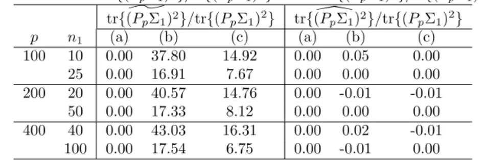
From these simulation results, we can see that our tests are more robust against the effects of non-normality as compared to Harrar and Kong’s test. The difference between Harrar and Kong’s test and our test appears in the estimator of tr{(PgΣg)²}. Thus, we compare the bias of Harrar and Kong’s estimatortr{(P^pΣg)²}divided by the true parameter tr{(PgΣg)²}and one of our estimatorstr{(P\pΣg)²}divided by the true parameter tr{(PgΣg)²}under the model (4.1) with µg = 0 andΣg = (1−0.5)Ip +0.51p1^⊤_p. The biases of these estimators are calculated using 10,000 replications in each setting. The biases oftr{(P^pΣg)²}/tr{(PgΣg)²}andtr{(P\pΣg)²}/tr{(PgΣg)²}are presented in Table 5. The settings ofpandngcan be checked in Table 5.

Please insert Table 5 approximately here.

From Table 5, we can see thattr{(P^_pΣg)²}remarkably overestimates tr{(P_pΣg)²}when the distribution ofZg jis (b) or (c). This overestimation contributes to raising the critical value of the test. Since raising the critical value is equivalent to difficulty in rejecting the null hypothesis, we expect that the size for Harrar and Kong’s test will be lower than the nominal significance level. This observation is consistent with the results of Table 2. On the other hand, we can understand thattr{(P\pΣg)²}is almost unaffected by change in distribution. Therefore, we can understand that changing the estimator of tr{(PpΣg)²}is never a minor correction.

4.2. Real example

We apply our test to the following dataset analyzed by Takahashi and Shutoh [13]. The data consist of a = 2 groups, with a body weight ofn_g=10 rats for each group. The weights of the total 20 rats were observed every week forp=22 weeks.

We applied our tests (3.5) and (3.6) to the parallelism hypothesisH01and flatness hypothesisH02with the signif- icance levelα=0.05. SinceT01/√

b

σ²_H01andz_αare calculated as T01/√

b

σ²_H01 ≈ −0.657<z_α≈1.6449, we can see that the parallelism hypothesisH01is retained. SinceT₀₂/√

b σ²_H

02 andz_αare calculated as T₀₂/√

b σ²_H

02 ≈250.264>z_α≈1.6449, we can see that the flatness hypothesisH02is rejected.

5. Discussion and Conclusion

In this paper, we proposed new approximation tests for the parallelism and flatness hypotheses in profile analysis for high-dimensional elliptical populations with unequal covariance matrices, and we derived the asymptotic sizes and power of these proposed tests. We showed that the asymptotic sizes of the proposed tests are at a nominal signifi- cance level. However, Harrar and Kong’s approximation tests do not necessarily have similar properties for elliptical populations, because the unbiasedness of their estimator of asymptotic variance depends on kurtosis parameters. Fur- thermore, we found that the asymptotic power depends on the value obtained by dividing the distance between the null and alternative hypotheses by the variance under the alternative hypothesis.

Furthermore, we compared the proposed tests and Harrar and Kong’s tests numerically in simulation studies. We found that our tests and Harrar and Kong’s tests had approximately the same accuracy when the population distribution is a multivariate normal distribution, and we confirmed our expectation that our tests are superior to Harrar and Kong’s tests for elliptical distributions other than the multivariate normal distribution. We also confirmed that this superiority is attributable to the estimator used in asymptotic variance.

In addition, we applied the tests to real data. However, we have not determined whether the assumption of an elliptical population is appropriate. The solution to this problem is to find the validity of the elliptical distribution from the data or to guarantee accuracy with a wider range of distribution families than the elliptical distribution. To achieve the former, it is necessary to extend the method proposed by Batsidis and Zografos [1] to high-dimensional settings.

To achieve the latter, it will first be necessary to investigate situations in which the symmetry of the distribution is not assumed, such as when a skew elliptical distribution is used. This change is expected to complicate the estimation of the asymptotic variance. These two tasks are left to future work.

Acknowledgments

We would like to thank Mr. Ogawa for the Monte Carlo simulation used to obtain the numerical results. We also would like to thank the Editor-in-Chief, an Associate Editor, and two reviewers for many valuable comments and helpful suggestions which led to an improved version of this paper. The research of the author was supported in part by a Grant-in-Aid for Young Scientists (B) (17K14238) from the Japan Society for the Promotion of Science.

8

References

[1] A. Batsidis, K. Zografos A necessary test of fit of specific elliptical distributions based on an estimator of Song’s measure,J.Multivariate Anal.,113(2013) 91–105.

[2] S. X. Chen, Y.-L. Qin, A two-sample test for high-dimensional data with applications to gene-set testing,Ann. Statist.38(2010) 808–835.

[3] P. Hall, C.C. Heyde,Martingale Limit Theory and its Application, Academic Press, New York, 1980.

[4] S. W. Harrar, X. Kong, High-dimensional multivariate repeated measures analysis with unequal covariance matrices,J.Multivariate Anal., 145(2016) 1–21.

[5] T. Himeno, T. Yamada, Estimations for some functions of covariance matrix in high dimension under non-normality and its applications.J.

Multivariate Anal.,130(2014) 27–44.

[6] Y. Kano An asymptotic expansion of the distribution of Hotelling’sT²-statistic under general distributions.Amer. J. Math. and Manage. Sci., 15(1995) 317-341.

[7] Y. Maruyama, Asymptotic expansions of the null distributions of some test statistics for profile analysis in general conditions,J.Statist.

Plann.Inference,137(2007) 506–526.

[8] A.M. Mathai, S.B. Provost, T. Hayakawa,Bilinear forms and zonal polynomials, Lecture Notes in Statistics, 102, Springer-Verlag, New York, 1995.

[9] R. J. Muirhead,Aspects of Multivariate Statistical Theory, John Wiley & Sons, Inc., New York (1982).

[10] N. Okamoto, N. Miura, T. Seo, On the distributions of some test statistics for profile analysis in elliptical populations,Amer. J. Math. Manag.

Sci.,26(2006) 1–31.

[11] A.N. Shiryaev,Probability, second ed., Springer-Verlag, 1984.

[12] M. S. Srivastava, Profile analysis of several groups,Commun. Stat.-Theory Meth.,16(3) (1987) 909–926.

[13] S. Takahashi, N. Shutoh, Tests for parallelism and flatness hypotheses of two mean vectors in high-dimensional settings,J.Stat. Com- put.Simul.,86(2016) 1150–1165.

A. Appendix A.1. Some moments

Lemma A.1. Let beX∼ Cp(ξ,0,Λ), and let A and B be p×p symmetric real matrices.

(i) E(X^⊤AX)=tr(AΣ),

(ii) E(X^⊤AXX^⊤BX)=(κ+1){tr(AΣ)tr(BΣ)+2tr(AΣBΣ)}, (iii) var(X^⊤AX)=κ{tr(AΣ)}²+2(κ+1)tr(AΣ)²,

(iv) cov(X^⊤AX,X^⊤BX)=κtr(AΣ)tr(BΣ)+2(κ+1)tr(AΣBΣ), where

Σ:=−2ξ^′(0)Λ, κ:= ξ^′′(0) (ξ^′(0))² −1

(

=E{(X^′Σ⁻¹X)²} p(p+2) −1

) . Proof. See Mathai et al. [8].

A.2. Proof of Lemma 2.1

We defineYgi = Xgi−µgforg∈ {1, . . . ,a},i∈ {1, . . . ,ng}. Note thatYgiis distributed according to an elliptical distribution with E(Ygi)=0and var(Ygi)= Σg.

Then the statisticT can be rewritten as T =

∑a g=1

dg

n_g(n_g−1)

n_g

∑

ii=1,j

Y^⊤_giPpYg j+

∑a g,h

ψδgδhY^⊤_gPpYh+2µ^⊤(Ra⊗Pp)Y+µ^⊤(Ra⊗Pp)µ,

whereY = (Y^⊤₁, . . . ,Y^⊤_a)^⊤. We note thatµ^⊤(R_a⊗P_p)Y =0 andµ^⊤(R_a⊗P_p)µ=0 if (R_a⊗P_p)µ=0. That is, the distribution ofT does not depend onµas long as (R_a⊗P_p)µ=0.

Letn₍₀₎=0,n_(g)=∑g

ℓ=1n_ℓforg∈ {1, . . . ,a}, andi^′=i−n_(g−1). We define

εi= 2

σn_g(n_g−1)Y^⊤_gi′P_pagi^′

forg∈ {1, . . . ,a}, i∈ {n(g−1)+1, . . . ,n(g)}. Here, agi^′=I(i^′≥2)d_g

i^′−1

∑

j=1

Yg j+I(g≥2)(n_g−1)

g−1

∑

h=1

ψδgδhYh+(n_g−1)

∑a h=1

ψδgδhµh,

whereI(·) denotes an indicator function. Then,

T−µ^⊤(Ra⊗Pp)µ

σ =

n(a)

∑

i=1

εi.

DefineF0={∅,Ω}, and letFifori∈Nbe theσ-algebra generated by the random variables (ε1, . . . , εi). Then we find that

F0⊆ · · · ⊆ F_∞ and E(εi|Fi−1)=0. Thus,{εi}is a martingale difference sequence.

We show the asymptotic normality of ∑n_(a)

i=1εi by adapting the martingale difference central limit theorem (see Shiryaev [11] or Hall and Heyde [3]). It is necessary to check the following two conditions to apply this theorem:

(I)

n_(a)

∑

i=1

E(ε²i|Fi−1)=1+op(1) asp→ ∞,

(II)

n_(a)

∑

i=1

E(ε⁴i)=o(1) asp→ ∞ 10

under (A1), (A2), and (A3).

First, we check condition (I). We rewrite

n_(a)

∑

i=1

E(ε²i|Fi−1)=1+

∑7 j=1

Aj,

where

A₁ =

∑a g=1

4d²_g σ²n²_g(ng−1)²

n_g

∑

i=1

(n_g−i)[Y^⊤_giP_pΣgP_pYgi−tr{(ΣgP_p)²}],

A2 =

∑a g=1

8d²_g σ²n²_g(n_g−1)²

n_g

∑

i=2 i−1

∑

j=1

(ng−i)Y^⊤_giPpΣgPpYg j,

A₃ =

∑a g=2

g−1

∑

h=1

8dgψδgδh

σ²n²_g(ng−1)

n_g

∑

i=1

(n_g−i)Y^⊤_giP_pΣgP_pYh,

A4 =

∑a g=1

∑a h=1

8dgψδgδh

σ²n²_g(ng−1)

n_g

∑

i=1

(ng−i)Y^⊤_giPpΣgPpµh,

A₅ =

∑a g=2

g−1

∑

h=1

4ψ²δ²gδ²_h σ²ng

{

Y^⊤_hP_pΣgP_pYh−tr(P_pΣgP_pΣh) nh

} ,

A6 =

∑a g=3

g−1

∑

h=2 h−1

∑

ℓ=1

8ψ²δ²gδhδ_ℓ ng

Y^⊤_hPpΣgPpY_ℓ,

A7 =

∑a g=2

g−1

∑

h=1

∑a ℓ=1

8ψ²δ²gδhδℓ

σ²ng

Y^⊤_hPpΣgPpµ_ℓ.

It is straightforward to show that E(∑7

j=1Aj)=0. Holder’s inequality yields var



n_(a)

∑

i=1

E(ε²i|Fi−1)

=E







∑7 i=1

Ai





2

≤7

∑7 i=1

E(A²_i). (A.1)

The expectations E(A²₁) through E(A²₇) are evaluated as follows:

E(A²₁) ≤

∑a g=1

2(2ng−1)(3κg+2)

3n_g(n_g−1) =o(1), (A.2)

E(A²₂) ≤

∑a g=1

4(ng−2) 3ng

tr{(PpΣg)⁴}

[tr{(PpΣg)²}]² =o(1), (A.3)

E(A²₃) ≤

∑a g=2

g−1

∑

h=1

2(2ng−1) 3ng

√

tr{(PpΣg)⁴} [tr{(P_pΣg)²}]²

√

tr{(PpΣgPpΣh)²}

{tr(P_pΣgP_pΣh)}² =o(1), (A.4) E(A²₄) ≤

∑a g=1

2(2n_g−1) 3ng

√

tr{(P_pΣg)⁴}

[tr{(PpΣg)²}]² =o(1), (A.5)

E(A²₅) ≤ a(a−1)

∑a g=2

a−1

∑

h=1

[ κh

2n_h +(κh+nh)tr{(PpΣgPpΣh)²} n_h{tr(P_pΣgP_pΣh)}²

]

=o(1), (A.6)

E(A²₆) ≤ a(a−1)(a−2)

∑a g=3

g−1

∑

h=2 h−1

∑

ℓ=1

2√

tr{(PpΣgPpΣh)²}tr{(PpΣgPpΣℓ)²}

3tr(P_pΣgP_pΣh)tr(P_pΣgP_pΣ_ℓ) =o(1), (A.7) E(A²₇) ≤ a(a−1)

∑a g=2

g−1

∑

h=1

√tr{(PpΣgPpΣh)²}

tr(PpΣgPpΣh) =o(1). (A.8)

The details of these inequalities are described in Supplemental Materials 1. Substituting (A.2)-(A.8) into (A.1) yields var



n(a)

∑

i=1

E(ε²i|Fi−1)

=o(1). Condition (I) follows.

Next, we check condition (II). Define ε⁽¹⁾_i = 2I(i^′≥2)dg

σn_g(n_g−1)Y^⊤_gi′P_p

i^′−1

∑

j=1

Yg j, ε⁽²⁾_i =2I(g≥2) σn_g Y^⊤_gi′P_p

ℓ−1

∑

h=1

ψδgδhYh, ε⁽³⁾_i = 2 σn_gY^⊤_gi′P_p

∑a h=1

ψδgδhµh.

Then, Holder’s inequality yields

n_(a)

∑

i=1

E(ε⁴i)=

∑a g=1

n_(g)

∑

i=n_(g−1)+1

E







∑3 j=1

ε⁽_i^j)





4

≤

∑a g=1

n_(g)

∑

i=n_(g−1)+1

E



3³

∑3 j=1

ε⁽_i^j)4



=3³

∑a g=1

n_(g)

∑

i=n_(g−1)+1

∑3 j=1

E (ε⁽_i^j)4)

.

Thus, it is sufficient to show that∑n_(g)

i=n_(g−1)+1E(ε⁽_i^j)4)=o(1) forj∈ {1,2,3}. We have following expectations:

n(g)

∑

i=n_(g−1)+1

E (ε⁽¹⁾_i ⁴)

≤ 18(κg+1)²

ng(ng−1) +4(κg+1)(n_g−2)

ng(ng−1) +8(κg+1)(n_g−2)

ng(ng−1) =O(n⁻_g¹),

n(g)

∑

i=n_(g−1)+1

E (ε⁽²⁾_i ⁴)

≤

g−1

∑

h=1

9(κg+1)(κh+1) ngnh +

g−1

∑

h=1

3(κg+1)(nh−1) ngnh +

g−1

∑

h,h^′

3(κg+1) ng +

g−1

∑

h,h^′

6(κg+1)

ng =O(n⁻_g¹),

n(g)

∑

i=n_(g−1)+1

E (ε⁽³⁾_i ⁴)

≤ 3

ng =O(n⁻_g¹).

The details of these inequalities are described in Supplemental Materials 2. The above results complete the proof of (II).□

A.3. Proof of Lemma 3.1

First, we show the unbiasedness and consistency oftr(P\_pΣg)². From Lemma A.1, it follows that E[tr{(P_pS_g)²}] = κg+1

ng

[{tr(P_pΣg)}²+2tr{(P_pΣg)²}]

+n²_g−2ng+2

ng(ng−1) tr{(P_pΣg)²}+ 1

ng(ng−1){tr(P_pΣg)}², E[{tr(PpSg)}²] = κg+1

n_g

[{tr(PpΣg)}²+2tr{(PpΣg)²}]

+ 2

n_g(n_g−1)tr{(PpΣ