PAPER
A State Space Compression Method Based on
Multivariate Analysis for Reinforcement Learning in
High-dimensional Continuous State Spaces
Hideki SATOH†a), Member
SUMMARY A state space compression method based on multivariate analysis was developed and applied to reinforcement learning for high-dimensional continuous state spaces. First, use-ful components in the state variables of an environment are ex-tracted and meaningless ones are removed by using multiple re-gression analysis. Next, the state space of the environment is compressed by using principal component analysis so that only a few principal components can express the dynamics of the envi-ronment. Then, a basis of a feature space for function approxima-tion is constructed based on orthonormal bases of the important principal components. A feature space is thus autonomously con-struct without preliminary knowledge of the environment, and the environment is effectively expressed in the feature space. An example synchronization problem for multiple logistic maps was solved using this method, demonstrating that it solves the curse of dimensionality and exhibits high performance without suffer-ing from disturbance states.
key words: reinforcement learning, curse of dimensionality, multivariate analysis, approximation, nonlinear
1. Introduction
Reinforcement learning [1] has been receiving much at-tention because it can construct, without a supervisor or a model of an environment, a control function that computes an action based on the state variables of the environment. To apply reinforcement learning to the real world, we need to extend it to high-dimensional continuous state spaces because most problems in the real world comprise high-dimensional continuous states. However, as the dimension of the state space increases, the dimension of a feature space, in which a nonlin-ear control function is approximated, increases expo-nentially [1]. That is, the number of parameters to be learned increases exponentially. This is referred to as the “curse of dimensionality” and is one of the most serious problems in function approximation and rein-forcement learning.
To approximate a nonlinear control function and to solve the curse of dimensionality, various approaches to autonomously constructing a feature space have been investigated. In the wire fitting approach, a feature
Manuscript received December 22, 2005. Manuscript revised April 4, 2006. Final manuscript received April 17, 2006.
†The author is with the Future University-Hakodate,
Hakodate-shi, 041-8655 Japan. a) E-mail: [email protected]
space for function approximation is constructed based on the control wires, that fit the control surface and create the relationship between the state and the ac-tion. Restricting the number of control wires enables the optimal action for a given state to be quickly found and reduces the number of parameters to be learned [2]. Tile coding with hashing allocates tiles whose position and size are randomly selected in a state space, and uses the tiles as a basis that constructs a feature space. By restricting the number of tiles, tile coding compresses the state space [1]. A tree-based algorithm has been de-veloped that can handle a large continuous state space [3]. The self-organising map can perform function ap-proximation autonomously in a feature space with a limited dimension [4]. These methods aim at effective construction of a feature space for function approxi-mation. However, their function approximations are redundant because the basis of the feature space is not orthogonal. Because the mathematical structure of the feature space is unclear, it is difficult to ensure impor-tant properties such as the stability of the system. Hi-erarchical reinforcement learning is another approach to solving the curse of dimensionality. It constructs a hierarchical structure in the environment and controls each level in the hierarchy by using multiple agents. The number of parameters that each agent has to learn is reduced by dividing the state space based on the hi-erarchical structure [5], [6]. However, because prelimi-nary knowledge is required in most cases to construct a hierarchical structure, it is difficult to apply hierar-chical reinforcement learning to an environment whose structure is unknown. It is also difficult to mathemat-ically clarify the demand and reason for constructing the structure.
In this paper, a method is presented that solves these problems and the curse of dimensionality. It is a state space compression method that uses multi-variate analysis. It autonomously constructs a feature space without preliminary knowledge of the environ-ment. It is based on orthogonal bases, so the mathe-matical structure of the system is clear in the feature space, and it is possible to mathematically analyze the dynamics and stability in a moment vector space [7]. Its ability to solve a synchronization problem for multiple logistic maps [8] using reinforcement learning
demon-strated that the state space compression method us-ing multivariate analysis exhibits high performance and solves the curse of dimensionality.
2. Actor-critic Method for Continuous-state
Continuous-action Environment 2.1 Reinforcement Learning
A system with reinforcement learning [1] comprises two elements: an agent and an environment. The former provides a control function, and the latter denotes the target system to be controlled. The agent observes the state variables and the reward from the environment, updates the control function accordingly, and outputs a new control input to the environment. The control function and control input are referred to as policy and action, respectively.
Let us consider a discrete-time continuous-state continuous-action environment defined by a Markov de-cision process (MDP). Let u def= t(u
1, · · · , udu) be the action of dimension du, sdef= t(s1, · · · , sds) be the state of dimension ds, Dsdef= {si|smini≤ si≤ smini+Dsi, 1 ≤ i ≤ ds}, Dudef= {ui|umini ≤ ui ≤ umini+ Dui, 1 ≤ i ≤ du}, r be the immediate reward, and superscript t
de-note transposition. In an MDP environment, transition probability density function prob(st+1|st, ut) is defined
to describe the relationships among st, ut, and st+1,
and rtis given when the agent takes action utand the
state changes from stto st+1. Here subscript t denotes
the discrete time.
Reinforcement learning differs from supervised learning, such as neural networks, machine learning, and statistical pattern recognition. Without any help from a supervisor, it maximizes discount return Rt
de-fined by Rt def= tXmax k=0 νDRkr t+k+1 for 0 < tmax≤ ∞ = rt+1+ νDRRt+1, (1)
where νDR is the discount rate (0 ≤ νDR ≤ 1).
Actor-critic methods [9], [10], which is a class of methods for solving reinforcement learning problems, consist of two parts: an actor and a critic. The actor observes state
st and decides on action ut based on policy p(ut|st),
which denotes the conditional probability density func-tion (PDF) of ut. The critic observes rt, updates
state-value function V (s)def= E[Rt|st = s] accordingly, and
learns policy p(u|s).
2.2 Function Approximation
Function approximation is essential for reinforcement
learning in a continuous-state continuous-action envi-ronment. It constructs an approximation of a nonlin-ear function. In this section, linnonlin-ear function approxi-mations [1] are summarized that approximately express
V (s) and p(u|s).
State-value function V (s) is approximated by
V (s, c), which is defined by the following expansion: V (s, c) def= NV X i=0 ciφVi(s) = tc · φV(s), (2)
where NVdenotes the degree of expansion of V (s), cdef= t(c
0, · · · , cNV), and φV(s)
def
= t(φ
V0(s), · · · , φVNV(s)). Here, an orthonormal basis described in Appendix A is used for φV(s). An NV+ 1 dimensional vector space
with basis φV(s) is referred to as a feature space. From Eq. (2), V (s) is expressed by vector c in the feature space with basis φV(s).
To simplify approximation of p(u|s), let us assume that ui obeys a normal distribution and that ui and
uj are independent for i 6= j. Then, p(u|s) can be
approximated by the following equation:
p(u|s) ∼= du Y i=1 pG(ui|s, ξmi, ξσ i), (3) pG(ui|s, ξmi, ξσ i) def = 1 (2π)1/2σG(s, ξσ i) exp(−(ui− mG(s, ξmi)) 2 2σG(s, ξσ i)2 ),
where mG(s, ξmi) denotes an approximation of the mean of ui when the state of the environment is s,
σG(s, ξσ i) denotes an approximation of the standard deviation of ui when the state of environment is s,
ξmi def= t(ξ
mi0, · · · , ξmiNm), ξσ i
def
= t(ξ
σ i0, · · · , ξσ iNσ),
Nm denotes the degree of expansion of mG, and Nσ denotes the degree of expansion of σG.
Let φm(s) def
= t(φ
m0(s), · · · , φmNm(s)) be an or-thonormal basis. In the same manner as the approxi-mation of V (s), mG(s, ξmi) is defined as follows:
mG(s, ξmi) def
= tξ
mi· φm(s). (4)
Because σG(s, ξσ i) is positive, it cannot be directly
ex-panded using an orthonormal basis, as in Eqs. (2) and (4). Thus, the following function approximation is used to transform a variable expanded by an orthonormal function expansion into a positive number:
σG(s, ξσ i) def = ( σ˜umax− ˜σumin 1 + exp(−tξ σ i· φσ(s)) + ˜σumin)Dui, (5) where φσ(s)def= t(φ σ 0(s), · · · , φσ Nσ(s)) is the
are given by ˜σuminDuiand ˜σumaxDui, respectively.
Us-ing these function approximations enables the mean of
ui to be expressed by vector ξmi in a feature space
with basis φm(s) and the standard deviation of ui to
be expressed by vector ξσ iin a feature space with basis
φσ(s).
2.3 Actor-critic Method
Let εTDt, ct, ξmi;t, and ξσ i;t be the values of TD error
εTD [1], c, ξmi, and ξσ i at time t, respectively. An actor-critic method based on TD learning [1] and on the function approximations derived in Sect. 2.2 is given as follows:
Algorithm 1: Actor-critic method.
(1-1) Initialization-1: Set c0, ξmi;0, and ξσ i;0for ∀i.
(1-2) Initialization-2: Set t = 0, s0, and u0.
(1-3) Environment: Receive ut, and output rt+1 and
st+1to the agent.
(1-4) Actor-critic:
(1) Critic-1: Calculate εTDt and ct+1 by using Eqs.
(9) and (11) (Update V (s, c)).
(2) Critic-2: Calculate ξmi;t+1, ξσ i;t+1 by using Eqs. (12) and (13) (Update pG(ui|s, ξmi, ξσ i)) for ∀i.
(3) Actor: Set ui;t+1based on pG(ui;t+1|st+1, ξmi;t+1,
ξσ i;t+1) for ∀i.
(1-5) Set t = t + 1. If an episode finished, go to Step (1-2), else go to Step (1-3).
Here, episode denotes a trial [1]. In Step (1-1), initial values c0, ξmi;0, and ξσ i;0 are set for ∀i as follows:
c0= 0, ξmij;0= ½ umini+ Dui/2 for j = 0 0 for 1 ≤ j ≤ Nm, ξσ ij;0= ½ ξ0 for j = 0 0 for 1 ≤ j ≤ Nσ,
where ξ0 is set so that σG(s, ξσ i) takes an appropriate value for initial learning. In Sect. 5, ξ0 is set to −1.0
for ∀i, so that σG(s0, ξσ i;0) = 0.135Dui.
Let p(s) be the PDF of s and MSE(c) be the mean square error (MSE) of state-value function V (s) defined by
MSE(c)def= Z
s∈Ds
p(s)(V (s) − V (s, c))2ds. (6)
A method [1] that minimizes MSE(c) with respect to
c and updates V (s, c) is summarized below. Let ˆV (s)
be an estimation of the state-value function. We can obtain ˆV (s) by using the following equation:
ˆ
V (st) = rt+1+ νDRV (st+1, ct). (7)
Thus, by replacing x with s, ζ with ζV, g with V , and ˆg with ˆV in Eq. (A· 8), we obtain the following equation: ct+1= ct+ ζV( ˆV (st) − V (st, ct))∇cV (st, ct), (8) where ζV is the step size. By substituting TD error
εTDt, defined by
εTDt
def
= ˆV (st) − V (st, ct)
= rt+1+ νDRV (st+1, ct) − V (st, ct), (9) and ∇cV (s, c) = φV(s) into Eq. (8), we obtain
ct+1= ct+ ζVεTDtφV(st). (10) Let νTr be the trace-decay parameter [1]. By introduc-ing eligibility trace ηt [1] into the above equation, we
obtain the following equation for updating c:
ηt= νDRνTrηt−1+ φV(st),
ct+1= ct+ ζVεTDtηt. (11)
Here, η0, the initial value of ηt, is set to 0.
In the same manner as for V (s, c), pG(ui|s, ξmi, ξσ i)
can be updated. Let ζmbe the step size to update ξmi;t,
and ζσ be the step size to update ξσ i;t. By replacing
ct with ξmi;t, ˜g with ui;t, g(xt, ct) with mG(st, ξmi;t),
and ∇cg(x, c) with ∇ξmiξmi· φm(st) = φm(st) in Eq. (A· 9), we obtain the following equation:
ξmi;t+1 = ξmi;t
+ζmεTDt(ui;t− mG(st, ξmi;t))φm(st). (12)
In the same manner as for Eq. (12), by replacing ct
with ξσ i;t, ˜g with |ui;t− mG(st, ξmi;t)|, g(xt, ct) with
σG(st, ξmi;t), and ∇cg(x, c) with ∇ξσ iξσ i · φσ(st) =
φσ(st) in Eq. (A· 9), we obtain the following equation:
ξσ i;t+1 = ξσ i;t+ ζσεTDt(|ui;t− mG(st, ξmi;t)|
−σG(st, ξσ i;t))φσ(st). (13)
3. State Space Compression Method and its
Application to Reinforcement Learning 3.1 Framework of State Space Compression and
Learning
Let us consider a system in which several controllers control an environment, and assume that the agent is one of the controllers. The controllers observe the state variables and the reward from the environment, and output control inputs to the environment. Sup-pose that the agent can observe state xt, reward rt+1,
and control input vt that includes control inputs
de-termined by the other controllers and action ut
deter-mined by the agent. Note that it is assumed that xtand
vtdoes not not always include all the states in the
other controllers. To simplify the equations described later, the relationship between ut and vt is defined as
follows: ut= Guvt+ gu. (14) Here, xtdef= t(x1;t, · · · , xdx;t), vt def = t(v 1;t, · · · , vdv;t), Dx def
= {xi |xmini≤ xi ≤ xmini+ Dxi, 1 ≤ i ≤ dx}, Dv def= {vi |vmini≤ vi≤ vmini+ Dvi, 1 ≤ i ≤ dv}, and Gu and gu are a matrix and a vector, respectively, obtained
from vmini, Dvi, umini, and Dui.
When the basis of x for function approximation is constructed using the direct product of the bases of
xi, the degree of expansion of x increases
proportion-ally to the dxth power of the degree of expansion of xi (see Eq. (A· 4)). This is referred to as the “curse
of dimensionality.” The framework of state space com-pression and reinforcement learning presented in this section solves this problem. In the framework, the agent compresses the state space, constructs a feature space with a limited dimension, extracts the principal dynamics in xt, and determines ut. The procedure
op-erated by the agent is summarized as follows (the num-bers in parentheses correspond to (1), · · ·, (7) in Step (2-4) of Algorithm 2). (3) Compute statistics such as mean and covariance of x. (4) Compute the resolution (which denotes the importance) of xi using multiple
regression analysis. Based on the resolution, extract useful components of x and remove meaningless ones. (5) Compute principal axes matrix M , which maps the useful components of x to principal component vector
y =t(y
1, · · · , ydy), which express the principal dynam-ics in the useful components of x. (6) Compute the resolution of yi. (7) Based on the resolution of yi,
de-termine bases φV, φm, and φσ. (1) Transform x into
y using principal axes matrix M , and normalize y into
normalized principal state s so that s contains the prin-cipal dynamics in x in a bounded space. (2) Compute action u based on s using the actor-critic method in the feature spaces with bases φV, φm, and φσ.
In the above procedure, it is necessary, before per-forming the actor-critic method, to obtain principal axes matrix M , bases φV, φm, and φσ, and normalized principal state s. Thus, before performing the actor-critic method, u is determined at random, and statis-tics such as the mean and covariance of x are computed. After a sufficiently long time has elapsed, M , φV, φm,
and φσ are computed. They are updated at appropri-ate intervals so that they include the lappropri-atest dynamics in the environment. The time when M , φV, φm, and φσ are computed is indicated by using two variables: nMA and trgMA. The former denotes the number of times
M , φV, φm, and φσ have been updated, and the
lat-ter denotes the trigger to update M , φV, φm, and φσ. Here, M , φV, φm, and φσare updated at regular
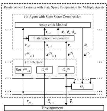
inter-val TRB. The structure and algorithm for the agent are
shown in Fig. 1 and given by Algorithm 2, respectively.
Fig. 1 Structure of agent with state space compression.
Algorithm 2: Reinforcement learning with state space compression.
(2-1) Initialization-1: Set trgMA= 0, nMA = 0, c0, ξm0,
and ξσ 0.
(2-2) Initialization-2: Set t = 0, x0, and u0.
(2-3) Environment: Receive ut, and output rt+1 and
xt+1 to the agent.
(2-4) Agent:
(1) Transform xt+1into st+1by using Eqs. (24) and
(32) if nMA ≥ 1.
(2) Perform actor-critic method (Step (1-4) in Al-gorithm 1) if nMA ≥ 1, or set ut randomly if
nMA = 0.
(3) Compute statistics of x, and set nMA and trgMA by using Algorithm 3.
(4) Compute resolution of state xi by using Eq. (20)
if trgMA= 1.
(5) Update principal axes matrix and mean by using Eqs. (23) and (25) if trgMA = 1.
(6) Compute resolution of yi by using Eq. (31) if
trgMA = 1.
(7) Update bases as shown in Sect. 3.7 and set
trgMA = 0 if trgMA = 1.
(2-5) Set t = t + 1. If an episode finished, go to Step (2-2), else go to Step (2-3).
Each step of the agent is described in detail below. 3.2 Statistics of Environment
To enable multivariate analysis to be performed, the mean and covariance of xt, xt+1, vt, and rt+1are
com-puted at appropriate intervals by using Algorithm 3 so that they include the latest dynamics in the environ-ment, where COVxx denotes the covariance matrix of
(x1;τ, · · · , xdx;τ), COVvxvx denotes the covariance ma-trix of (v1;τ, · · · , vdv;τ, x1;τ, · · · , xdx;τ), COVvxx0vxx0 de-notes the covariance matrix of (v1;τ, · · ·, vdv;τ, x1;τ,
· · ·, xdx;τ, x1;τ +1, · · ·,xdx;τ +1), covx0vxi
def
= t(cov(x
i;τ +1,
v1;τ), · · ·, cov(xi;τ +1, vdv;τ), cov(xi;τ +1, x1;τ), · · ·,
cov(xi;τ +1, xdx;τ)), covrvxx0
def
= t(cov(r
τ +1,v1;τ),· · ·, cov(rτ +1, vdv;τ), cov(rτ +1,x1;τ), · · ·, cov(rτ +1, xdx;τ),
cov(rτ +1,x1;τ +1),· · ·,cov(rτ +1,xdx;τ +1)), cov(xτ, yτ) de-notes the covariance of xτ and yτ, ¯x denotes the mean
of xτ, and t − TS+ 1 ≤ τ ≤ t.
Algorithm 3: Compute Statistics.
(3-1) Initialization: If nMA = 0, set T = TS. If nMA ≥ 0, set T = TRB.
(3-2) If the remainder of t + 1 upon division by T is equal to 0 (i.e., at periodic intervals of T ), perform the following steps.
(3-3) Compute COVxx, COVvxvx, COVvxx0vxx0, covx0vxi,
covrvxx0, and ¯x.
(3-4) Set nMA = nMA+ 1 and trgMA = 1.
Here, the statistics of x are initially computed at t =
TS− 1. Thereafter, the bases are updated at periodic
intervals of TRB.
3.3 Resolution of State xi
To determine action ut, it is necessary to estimate
which elements in state vector xt are important. The
resolution of xi;t for computing utis estimated by
us-ing the partial regression coefficients [11] and standard deviations.
First, the effect of vt and xton xt+1is estimated
by using the partial regression coefficients for xt+1. The
multiple regression equation [11] for criterion variable
xt+1with respect to explanatory variables vtand xtis
expressed by
xt+1= β0+ Bvvt+ Bxxt, (15)
where βi0, βvij, and βxij are the partial regression
co-efficients, β0 def = t(β 10, · · · , βdx0), βvi def = t(β vi1, · · · , βvidv), βxi def =t(β xi1, · · · , βxidx), Bv def = t[β v1, · · · , βvdx] is a dx × dv matrix, and Bx def= t[βx1, · · · , βxdx] is a
dx× dx matrix. Partial regression coefficients βvij and βxij are derived by the following equation [11]:
βvxi= COVvxvx−1covx0vxi, (16)
where βvxidef= t(tβ
vi,tβxi).
Next, the effect of vt, xt, and xt+1on rt+1is
es-timated by using the partial regression coefficient for
rt+1. The multiple regression equation for criterion
variable rt+1 with respect to explanatory variables vt,
xt, and xt+1 is expressed by
rt+1= b0+tbvvt+tbxxt+tbx0xt+1, (17)
where b0, bvj, bxj, and bx0jare the partial regression
co-efficients, bv def= t(bv1, · · · , bvdv), bx
def
= t(b
x1, · · · , bxdx), and bx0 def= t(bx01, · · · , bx0d
x). In the same manner as in Eq. (16), partial regression coefficients bvj, bxi, and bx0i
are derived by the following equation:
bvxx0 = (COVvxx0vxx0)−1covrvxx0, (18)
where bvxx0 def= t(tbv,tbx,tbx0).
Let resxvij be the resolution of xi for computing
vj. A combination of σ(xi), Dvj, |βvij|, and |bxi|+|bx0i|
is used to determine resxvij for three reasons:
(1) The effect of xi;t on vj;t denotes the agent itself.
Thus, if the effect of xi;t on vj;t is used to
deter-mine the resolution, a positive feedback loop arises, and a system with the agent may become unsta-ble. Thus, instead of the effect of xi;ton vj;t, |βvij|,
which denotes the effect of vj;t on xi;t+1, is used.
(2) Important information about the structure and dy-namics of the system are contained in σ(xi) and
σ(vj). However, σ(vj) contains the motion in the
agent, so the system may become unstable if σ(vj)
is used for the same reason described above. Thus,
Dvj instead of σ(vj) and σ(xi) are used.
(3) Because the agent works to obtain a large reward, it is effective to introduce |bxi| + |bx0i|, which
de-notes the effect of xi;t and xi;t+1 on rt+1.
Based on these reasons, resxvij is determined by resxvij= σ(xi)γ1Dvjγ2|βvij|γ3(|bxi| + |bx0i|)γ4, (19)
where γ1, · · · , γ4are given constants used to adjust the
combination. Here, σ(xi) = cov(xi, xi)1/2, and σ(xi) is
obtaind in Step (3-3) of Algorithm 3.
Let resxuibe the resolution of xiused for
comput-ing ut. As shown in Sect. 3.1, the relationship between
utand vtis defined by Eq. (14). Thus, resxuiis
deter-mined by the weighted sum of resxvijwith respect to j
as follows:
resxui=
du X
j=1
(Gut(resxvi1, · · · , resxvidx))j, (20)
where (·)j denotes entry j of a vector.
3.4 Principal Axes Matrix
As mentioned in Sect. 3.1, when the dimension of xt
is high, the degree of expansion of xt is too large to
perform reinforcement learning. Thus, it is necessary to express the dynamics in xt in a low-dimensional
feature space. In this section, principal components, which represent the important dynamics, are derived. Let yi;t be the ith principal component of xt, let ytbe
t(y
Sect. 3.5 and yi used for control is determined in Sect.
3.7. Thus, dy is set to dx.
Principal component vector yt is obtained as the
product of principal axes matrix M and state vector
xt, and M is derived from the eigenvector of COVxx
[11]. Most of the dynamics in xt can be expressed by
using only a small number of elements in yt if xi;t and
xj;t for i 6= j are correlated. However, it is not always
true that elements in xtwith large dynamics contribute
to reward rt+1. Some elements may not be related to
rt+1. To remove the effect of such elements on yt, the
covariance matrix for resxuixi is used instead of that
for xi. Let xRt def= t(resxu1x1;t, · · · , resxudxxdx;t) and
COVxxR be the covariance matrix of xR. From the def-inition of the covariance, COVxxR is obtained by using the elements of COVxx as follows:
COVxxR = [resxuiresxujcov(xi, xj)]. (21)
Let eR
i be the ith eigen vector of COV R
xx and M
R def
= [eR1, · · · , eRd
x] be the principal axes matrix of xRt. We then obtain principal component vector yt as follows:
yt = tMR
xR t
= tMRdiag[resxui]xt, (22)
where diag[resxui] denotes the diagonal matrix of resxui. Let principal axes matrix M of xt be defined
by the following equation:
M def= diag[resxui]M
R
. (23)
By substituting Eq. (23) into Eq. (22), we obtain
yt=tM xt. (24)
Let λi be the variance in yi;t, and ¯y be the mean of yt.
The former is equal to the ith eigen value of COVxxR,
and the latter is derived by ¯
y =tM ¯x. (25)
3.5 Resolution of State yi
As shown in Appendix A, bases φV, φm, and φσ are determined by the degree of expansion of yi. Thus, to
obtain a large discount return, it is reasonable to assign a larger value to the degree of expansion of yi;t if yi;t
is closely related to utand rt+1. The resolution of yi;t
is derived so as to achieve this aim in the same manner as in Sect. 3.3.
The multiple regression equation for yt+1 is
de-scribed in the same manner as in Eq. (15) as follows:
yt+1= ˜β0+ ˜Bvvt+ ˜Byyt, (26)
where ˜βi0, β˜vij, and ˜βyij are the partial
regres-sion coefficients, ˜β0 def = t( ˜β 10, · · · , ˜βdx0), β˜vi def = t( ˜β vi1, · · · , ˜βvidv), ˜βyi def = t( ˜β yi1, · · · , ˜βyidy), ˜Bv def = t[ ˜β v1, · · · , ˜βvdy] is a dy × dv matrix, and ˜By def = t[ ˜β y1, · · · , ˜βydy] is a dy× dy matrix. By substituting Eq. (24) into Eq. (15), we obtain
yt+1=tM β0+tM Bvvt+tM BxM yt. (27)
By comparing Eqs. (26) and (27), partial regression co-efficients ˜βvij is obtained by the following equation:
˜
Bv=tM Bv. (28)
By substituting Eq. (24) into Eq. (17), we can de-scribe the multiple regression equation for rt+1by using
rt+1 = b0+ bvvt+tbxM yt+tbx0M yt+1
= b0+ bvvt+tb˜yyt+tb˜y0yt+1. (29)
Here, tb˜
y def= ( ˜by1, · · · , ˜bydy) = tbxM and tb˜y0 def=
( ˜by01,· · ·, ˜by0d
y)=
tb
x0M . As a result, we obtain partial
regression coefficients ˜byi and ˜by0i from
˜
by =tM bx,
˜
by0 =tM bx0. (30)
Let resyvij be the resolution of yi for computing
vj and resyui be the resolution of yi for computing u.
In the same manner as in Eqs. (19) and (20), resyui is determined as follows:
resyui =
du X
j=1
(Gu(resyvi1, · · · , resyvidx))j, (31)
resyvij = σ(yi)˜γ1Dv˜γj2| ˜βvij|γ˜3(| ˜byi| + | ˜by0i|)˜γ4,
where ˜γ1, · · · , ˜γ4are given constants, and σ(yi) = λ1/2i .
3.6 State Transformation
Principal component vector yt obtained by using Eq.
(24) has a unique boundary because it is assumed that
xt∈ Dx, as mentioned in Sect. 3.1. However, ytdoes
not take all the values within the boundary. Thus, state vector stused by the actor-critic method is set by using
the following equation so that it is distributed over the whole feature space and expresses the dynamics in xt
as accurately as possible: si;t = Dsi 1 + exp(−yi;t− ¯yi cPNσ(yi) ) −Dsi 2 + ¯si, (32) where ds= dy, ¯si= smini+ Dsi/2, and cPN is set to 0.6 so that the first term on the right side of Eq. (32) is ap-proximately equal to the probability distribution func-tion of a normal distribufunc-tion with mean ¯yiand standard
3.7 Basis of Feature Space
Based on the resolution of yi obtained by using Eq.
(31), bases φV, φm, and φσare determined in this sec-tion. To simplify the algorithm, let NV, Nm, and Nσ
be set to N and let N be given in advance. Let NVi, Nmi, and Nσ i be set to Ni, let φV, φm, and φσ be set to φdef= t(φ
0, · · · , φN), and let φidef= K(x, k) as shown
in Eq. (A· 2) in Appendix A. Here, K(x, k) is a multi-dimensional orthonormal basis defined by Eq. (A· 1), k is the index vector, and the relationship between i, the index of the basis, and k is obtained by Eq. (A· 3).
Once N and K(x, k) are given, φ is determined by setting Ni. As mentioned in Sect. 3.5, to obtain a large
discount return, it is reasonable to assign a larger value to Ni if resyuiis large. Furthermore, Eq. (A· 4), which
shows the relationship between N and Ni, should hold.
Thus, to satisfy these requirements, we determine Ni
by the following equation:
Ni= int(α resyui), (33)
where int(·) denotes the integer part, and α is set so that |N −Qdy
i=1(Ni+ 1) − 1| is minimum for the given
N and resyui.
Let φ be the basis when the degree of expansion is
Nj, and φ0 be the basis when the degree of expansion
is N0
j. When the degree of expansion changes from Nj
to N0
j, the basis also changes from φ to φ0. Thus, new
coefficients c0, ξ0
mi0, and ξ0σ i0 for the new bases have
to take the values of the old ones, c, ξmi, and ξσ i, for learning to proceed smoothly. That is, c0
i0 is set to ci,
ξ0mi0 is set to ξmi, and ξσ i0 0 is set to ξσ i, if φ0i0 is equal
to φi. Further details are described in Appendix A.
4. Expansion to Multiple Agents
Let us consider an environment that L agents control, and in which the agents cannot always observe all the state variables and the control inputs. In this sec-tion, the agent described by Algorithm 2 is extended to multiple agents. Let ˆxi be the ith state variable
of the environment, ˆxdef= t(ˆx
1, · · · , ˆxdˆx) ∈ ˆDx, ˆDx def= {ˆxi|ˆxmini≤ ˆxi≤ ˆxmini+ ˆDxi, 1 ≤ i ≤ ˆdx}, ˆvibe the ith
control input of the environment, ˆv def= t(ˆv
1, · · · , ˆvdˆv), ˆ
Dv def= {ˆvi| ˆvmini≤ ˆvi ≤ ˆvmini+ ˆDvi, 1 ≤ i ≤ ˆdv}, r(`)
be the immediate reward that the `th agent receives,
x(`)t be the subset of ˆxtthat the `th agent can observe,
v(`)t be the subset of ˆvtthat the `th agent can observe,
and u(`)t be the action determined by the `th agent. To
express the relationship between x(`)t and ˆxt, and that
between v(`)t and ˆvt, let us introduce state observation
matrix Gs(`) and action observation matrix Gv(`). By
using Gs(`) and Gv(`), the `th agent observes x(`)t and
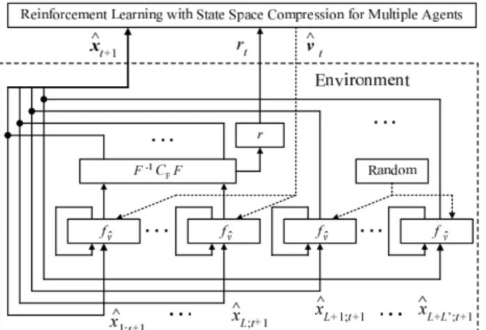
Fig. 2 Structure of reinforcement learning with state space compression for multiple agents.
v(`)t as follows:
x(`)t = Gs(`)xˆt,
v(`)t = Gv(`)ˆvt.
(34) Actions u(1)t , · · · , u(L)t are combined into ˆvtby
ˆ
vt= Gct(tu(1)t , · · · ,tu
(L)
t ) + gc. (35)
Here, Gc and gc are determined from vminiˆ , ˆDvi, umin(`)i , and Du(`)i . Immediate reward r
(`)
t for the `th
agent is set based on rt.
The structure and algorithm of reinforcement learning with state space compression for multiple agents are shown in Fig. 2 and given by Algorithm 4, respectively.
Algorithm 4: Reinforcement learning with state space compression for multiple-agents.
(4-1) Initialization-1: Set c(`)0 , ξm(`)0 , ξσ(`)0 , nMA(`)= 0, and trgMA
(`)= 0 for 1 ≤ ` ≤ L.
(4-2) Initialization-2: Set t = 0, ˆx0, and ˆv0.
(4-3) Environment: Receive ˆvt, and output ˆxt+1to the
interface.
(4-4) Interface: Set x(`)t+1, x(`)t , and v(`)t by using Eq.
(34) for 1 ≤ ` ≤ L, and set r(`)t+1for 1 ≤ ` ≤ L. (4-5) Agent with State Space Compression: Compute
u(`)t+1 by using Step (2-4) in Algorithm 2 for 1 ≤
` ≤ L.
Fig. 3 Simple environment: Linear combination of logistic maps.
(4-7) Set t = t + 1. If an episode finished, go to Step (4-2), else go to Step (4-3).
5. Performance Evaluation
Consider the simple example environment shown in Fig. 3, which is a linear combination of L + L0logistic maps
[8]. Here, du(`) = 1 for 1 ≤ ` ≤ L, ˆdv = dv = L, ˆdx = dx= L + L0, 0 ≤ ˆx`;t≤ 1 for 1 ≤ ` ≤ L + L0, I` is the
(` × `)-identity matrix, Gs(`) = IL+L0, Gv(`) = IL for
1 ≤ ` ≤ L, i.e., x(`)t = ˆxt and v(`)t = ˆvt for 1 ≤ ` ≤ L,
Gc = IL and gc = 0, i.e., ˆvt =t(u(1)1 t, · · · , u(L)1 t), and
the logistic map is defined by the following equation [8]:
x0 = f v(x)
def
= vx(1 − x). (36)
States ˆx0
1;t, · · ·, ˆx0L;t interact with each other, and ˆxt+1
is obtained by the following equation:
ˆ x0 `;t= nmaptimes z }| { fˆv`;t· · · fˆv`;t(ˆx`;t) for 1 ≤ ` ≤ L + L 0, t(ˆx 1;t+1, · · · , ˆxL;t+1) = F−1C FFt(ˆx01;t, · · · , ˆx0L;t), t(ˆx L+1;t+1, · · · , ˆxL+L0;t+1) =t(ˆx0 L+1;t, · · · , ˆx0L+L0;t), (37)
where nmap= 3, 3.4 ≤ ˆv`;t≤ 4 for 1 ≤ ` ≤ L + L0, F is
a matrix that performs discrete Fourier transform, and
CF def= diag[1.0, 0.9, 0.81, 0.73, 0.66, 0.59, 0.53, 0.48, · · ·],
which denotes a low pass filter that reduces the power spectrum of ˆx0
1;t, · · · , ˆx0L;t as the frequency increases.
The `th agent determines action u(`)1 t = ˆv`;t
by using the reinforcement learning described in Al-gorithm 4, and ˆvL+1;t, · · · , ˆvL+L0;t are set so that
they independently obey a uniform distribution. Let spc0;t, · · · , spcL−1;t be the power spectrum of
ˆ
x1;t, · · · , ˆxL;t, and immediate reward r(`)t+1for 1 ≤ ` ≤ L
be equal to rt+1 defined by rt+1def= (∆spck;t+1)2− L X j=1,j6=k (∆spcj;t+1)2, (38)
where the power spectrum denotes the square of the Fourier coefficients obtained by Ft(ˆx0
1;t, · · · , ˆx0L;t),
∆spcj;t+1
def
= spcj;t+1− spcj;t, k is set to 2. Thus, rt+1
increases when ˆx1;t, · · · , ˆxL;t move so that the motion
in spc2;t is large. Because ˆxL+1;t, · · · , ˆxL+L0;t are not
related to the immediate reward, they are disturbance states that disturb the 1st to the Lth agent.
The effectiveness of the state space compression algorithm described in Sect. 3 and the ability of Algo-rithm 4 to construct a feature space without being dis-turbed by the disturbance states were demonstrated by evaluating Algorithm 4 for various values for the degree of expansion, N , and the number of disturbance states,
L0, and for several combinations of γdef= (γ
1, γ2, γ3, γ4)
and ˜γdef= (˜γ1, ˜γ2, ˜γ3, ˜γ4). Note that the parameters for
each agent in Algorithm 4 have the same values, and superscript (`) for variables and parameters is omit-ted in the following to simplify the explanation. The combinations of γ and ˜γ evaluated were determined as
follows. (1) ˜γ1: It is reasonable to construct a feature
space based on the range of the ith principal compo-nent, yi. In other words, degree of expansion Ni for
yi should be proportional to σ(yi). Thus, ˜γ1 is set to
1. (2) γ2: Because it is clear that the difference in Dvj should be normalized, γ2 is set to 1. Note that γ2 does not affect the performance shown below,
be-cause du= 1 in the environment described in Eq. (37).
(3) γ3 and γ4: It is important to distinguish the states
that contribute to the reward from the states that dis-turb the control algorithm. To do this, the effect of
vj;t on xi;t+1 and those of xi;t and xi;t+1 on rt+1 are
evaluated. The former is expressed by |βvij|γ3, and the
latter is expressed by (|bxi| + |bx0i|)γ4. Thus, Algorithm
4 is evaluated for γ3 = 0 or 1, and γ4 = 0 or 1. (4) γ1, ˜γ2, ˜γ3, and ˜γ4: Because σ(xi) and σ(yi) express
the same property (i.e., the standard deviation in the state) of the environment, γ1is set to 0 so that an agent
does not take the standard deviation into account more than once. For the same reason, ˜γ2, ˜γ3, and ˜γ4 are set
to 0. Therefore, ˜γ is set to (1, 0, 0, 0), and γ is set to
(0, 0, 0, 0), (0, 1, 1, 0), (0, 1, 0, 1), or (0, 1, 1, 1), where the motions in Algorithm 4 for (0, 0, 0, 0) and (0, 1, 0, 0) are the same in the environment of Eq. (37), and (0, 0, 0, 0) means that resxu1 =, · · · , = resxuL+L0 = 1. The other
parameters for reinforcement learning are set as fol-lows: TS= 5 × 10⁶, TRB = 103, νTr = 0.3, νDR = 0.9, and ζV = ζm= ζσ= 10−4.
The effect of N and L on Algorithm 4 was esti-mated by evaluating the change in immediate reward
Fig. 4 Change in immediate reward for various values of degree of expansion after starting reinforcement learning (L = 8).
the state space compression in Algorithm 4 was demon-strated by also evaluating an algorithm that does not use the state space compression, in which M = I and
Ni was given in advance (N1 =, · · · , = NL = 1; i.e.,
N = 255 when L = 8). Figure 4 shows the change in rtfor L = 8 after starting reinforcement learning; that
is, the time in Figure 4 indicates t − TS. The figure
shows that Algorithm 4 with γ = (0, 0, 0, 0) provides a sufficiently large rt when N is at least 63. On the
other hand, Algorithm 4 without state space compres-sion (i.e., M = I) provides a lower value of rtalthough
N (= 255) is larger than 63. Therefore, the state space
compression method described in Sect. 3 is effective. Figure 5 shows the effect of N and L on rt, where rtis
normalized by the maximum value of rtfor each value of
L. The changes in the normalized reward for L = 4, 8,
and 16 are almost the same as shown in this figure. This means that the performance is not always affected by L, the dimension of the system. The factors af-fecting the performance could be the complexity of the environment defined by nmap and CF.
The effect of the number of disturbance states on immediate reward rtis shown in Fig. 6, where N = 255
and L = 8. This figure shows that the effect of γ3 and γ4becomes noticeable as L0, the number of disturbance
states, increases, and that the largest rt is obtained
when γ3= γ4= 1 for each value of L0. Thus, |βvij| and |bxi| + |bx0i| are effective to remove the effect of the
dis-turbance states, and we can conclude that Algorithm 4 with γ = (0, 1, 1, 1) constructs a feature space effec-tively and controls the environment without suffering the disturbance states.
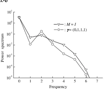
The motion in state ˆx`;twas demonstrated by
mea-suring the power spectrum and the change in state ˆ
x1;t, · · · , ˆxL;t for M = I and γ = (0, 1, 1, 1) after rt
was stable and saturated. The results are shown in Figs. 7 to 9 for N = 255, L = 8, and L0 = 0. The
origin of the time in Figs. 8 and 9 indicates the time
Fig. 5 The effect of N and L on normalized reward.
Fig. 6 Effect of number of disturbance states on immediate reward (N = 255 and L = 8).
when measurement started. These figures show that
spc2 in Eq. (38) is extracted and Algorithm 4 works well when γ = (0, 1, 1, 1), although ˆx1;t, · · · , ˆxL;t moves
almost randomly when M = I.
All combinations of γ and ˜γ were not evaluated,
and it was assumed that all states and control inputs in the environment could be observed. To better clar-ify the effectiveness of Algorithm 4, a more extensive investigation will be conducted.
6. Conclusion
A state space compression method based on multivari-ate analysis was developed and applied to reinforcement learning for high-dimensional continuous state spaces. It can autonomously construct a feature space without preliminary knowledge of the environment. An exam-ple synchronization problem for multiexam-ple logistic maps was solved, demonstrating that the state space com-pression method exhibits high performance without suf-fering from disturbance states. Because the basis of the
Fig. 7 Power spectrum of ˆx1, · · · , ˆx8 (N = 255, L = 8, and L0
= 0).
Fig. 8 Motion in ˆx1, · · · , ˆx8 for M = I (N = 255, L = 8, and
L0= 0).
Fig. 9 Motion in ˆx1, · · · , ˆx8for γ = (0, 1, 1, 1) (N = 255, L =
8, and L0 = 0).
feature space is orthogonal, the mathematical structure of the system in the feature space is clear, and it is possible to mathematically analyze the dynamics and stability in a moment vector space. The mathematical
analysis of the dynamics will be reported in a future.
Appendix A: Orthonormal Basis for Function
Approximation Let xdef= t(x
1, · · · , xdx) and Dx
def
= {xj|xminj ≤ xj ≤
xminj + Dxj, 1 ≤ j ≤ dx}. In this appendix, the
or-thonormal bases [12] for x ∈ Dxare summarized.
Let k def= t(k
1, · · · , kdx) be the index vector of the Fourier coefficient and h(k) be the Fourier coefficient for index vector k. The Fourier series expansion for function f (x) is defined by the following equation [12]:
f (x) = X k∈Z h(k)K(x, k), h(k)def= RD xf (x)K ∗(x, k)dx, where Z def= {kj|0 ≤ kj ≤ Nj, 1 ≤ j ≤ dx}, Nj is
the degree of expansion of xj, h(k) is the Fourier
coef-ficient, superscript ∗ denotes a complex conjugate, and
{K(x, k)} is a multi-dimensional orthonormal basis
de-fined by the following equation:
K(x, k)def=
dx Y
j=1
Kj(xj, kj). (A· 1)
Here, {Kj(xj, kj)} is one-dimensional orthonormal
ba-sis, Kj(xj, kj) is set to a trigonometrical function
de-fined by Kj(xj, kj)def= r 1 Dxj for kj= 0 r 2 Dxj sin( kj+ 1 2 ω0j(xj− xminj)) for kj ∈ No r 2 Dxj cos( kj 2 ω0j(xj− xminj)) for kj ∈ Ne ,
ω0jdef= 2π/Dxj, Ne denotes a set of even numbers, and Nodenotes a set of odd numbers.
Let us define basis φ(x) =t(φ
0(x), · · · , φN(x)) as
φi(x)def= K(x, k), (A· 2)
where i is the index of the basis, N is the degree of expansion of x, and N +1 is the dimension of the feature space with the basis. When Zdef= {kj|0 ≤ kj≤ Nj, 1 ≤
j ≤ dx}, that is, Z is a cube, the index of the basis is
obtained from index vector k as follows:
i = dx X j=1 kj dx Y ν=j+1 Nν. (A· 3)
From the degree of expansion of xj, we can obtain the
N =
dx Y
j=1
(Nj+ 1) − 1. (A· 4)
Given that the degree of expansion of xj is Nj,
suppose that the basis, the index of the basis, and the domain of k are given by φ, i(k), and Z, respectively. When the degree of expansion of xj is Nj0, φ0, i0(k),
and Z0are also given. As mentioned in Sect. 3.7, when
the degree of expansion changes from Nj to Nj0, the
new coefficients, c0
i0(k), ξ0mi0(k), and ξ0σ i0(k), for the new
bases take the values of the old ones, ci(k), ξmi(k), and ξσ i(k), as follows: c0 i0(k)= ci(k) for ∀k ∈ Z0, ξ0mi0(k)= ξmi(k) for ∀k ∈ Z0, ξ0σ i0(k)= ξσ i(k) for ∀k ∈ Z0. (A· 5) If k ∈ Z0 and k 6∈ Z, that is, there is no φ
i(k)
corre-sponding to φ0
i0(k), c0i0(k), ξmi0 0(k)j, and ξσ i0 0(k)j are set
to 0 .
Appendix B: TD Learning Based on Steepest
Descent Method
TD learning [1] based on the steepest descent method is summarized in this appendix. Let xdef= t(x
1, · · · , xdx),
Dx def= {xi|xmini≤ xi ≤ xmini+ Dxi, 1 ≤ i ≤ dx}, p(x)
be a PDF of x, g(x, c) be an approximation of func-tion g(x), and c be the parameter used by the approx-imation. Parameter c is determined so as to minimize
MSE(c) defined by MSE(c)def=
Z
x∈Dx
p(x)(g(x) − g(x, c))2dx. (A· 6)
Let us now derive parameter c by using the follow-ing steepest descent method [13].
Algorithm 5: Steepest Descent Method. (1) Set initial value c0 and step size ζ > 0.
(2) Set number of iterations t = 0. (3) ct+1= ct− ζ∇cMSE(ct).
(4) t = t + 1. (5) Go to Step (3).
Here, ctis the value of vector c at t.
To realize Step (3) in Algorithm 5, let us make the following assumption.
Assumption 1: PDF p(x) is the same as the PDF when Algorithm 5 has been performed.
By applying Assumption 1 and Eq. (A· 6) to Step (3) in Algorithm 5, and by replacing ζ with ζ/2, Step (3) in Algorithm 5 can be described as follows:
ct+1 = ct− (ζ/2)∇cMSE(ct)
= ct− (ζ/2)∇c(g(xt) − g(xt, ct))2
= ct+ ζ(g(xt) − g(xt, ct))∇cg(xt, ct). (A· 7)
Let ˆg(x) be the estimated value of g(x). When g(xt)
is unknown but ˆg(x) can be obtained, Step (3) of
Algo-rithm 5 is obtained by replacing g(x) with ˆg(x) in Eq.
(A· 7) as follows:
ct+1= ct+ ζ(ˆg(xt) − g(xt, ct))∇cg(xt, ct). (A· 8)
Consider that g(xt) is unknown and that we cannot
obtain ˆg(x); that is, we can obtain only an estimated
value, ˜g(x), of g(x) with unknown accuracy. In this
case, introducing TD error εTDt into Eq. (A· 7) and replacing g(x) with ˜g(x) enable Step (3) of Algorithm
5 to be expressed by the following equation:
ct+1= ct+ ζεTDt(˜g(xt) − g(xt, ct))∇cg(xt, ct). (A· 9)
References
[1] R. S. Sutton and A. G. Barto, Reinforcement Learning, MIT Press, USA, 1998.
[2] Baird, L. C. and Klopf, A. H., “Reinforcement learning with high-dimensional, continuous actions,” Technical Re-port WL-TR-93-1147, 1993.
[3] W. T. B. Uther and M. M. Veloso, “Tree based discretiza-tion for continuous state space reinforcement learning,”, Proceedings of AAAI-98, pp. 769–774, July, 1998. [4] A. J. Smith, “The applications of the self-organising map
to reinforcement learning,” Neural Networks archive, vol, 15, Issue 8-9 , pp. 1107–1124, Oct. 2002.
[5] T. Dietterich, “Hierarchical reinforcement learning with the MAXQ value function decomposition,” Journal of Artificial Intelligence Research, vol. 13, pp. 227–303, 2000.
[6] A. G. Barto and S. Mahadevan, “Recent advances in hi-erarchical reinforcement learning,” Discrete event dynamic systems, vol. 13, Issue 4, pp. 341–379, Oct., 2003. [7] H. Satoh, “Approximation and Analysis of Non-linear
Equations Based on Moment Vector Equation,” Tech. Rept. IEICE. NLP2005-1, pp. 1-6, Jan. 2005.
[8] E. Ott, Chaos in Dynamical Systems Second edition, Cam-bridge, UK, 2002.
[9] I. H. Witten, “An adaptive optimal controller for discrete-time Markov environments,” Information and Control, vol. 34, pp. 286–295, 1977.
[10] A. G. Barto, R. S. Sutton, and C. W. Anderson, “Neuron-like elements that can solve difficult learning control prob-lems,” IEEE Trans. on Systems Man and Cybernetics, vol. 13, pp. 835–846, 1983.
[11] R. A. Johnson, D. W. Wichern, Applied Multivariate Sta-tistical Analysis, 5th ed, Pearson Education (Prentice Hall USA), 2001.
[12] I. N. Bronshtein and K. A. Semendyayev, Handbook of Mathematics, Springer-Verlag, Berlin, 1997.
[13] W. H. Press, S. A. Teukolsky, W. T. Vetterling, and B. P. Flannery, Numerical Recipes in C 2nd Edition, Cambridge University Press, UK, 1992.