"Indirect" Time Series Analysis for One-Dimensional Chaos Based on Perron-Frobenius Operator: "Generalized" Ulam-Li's Approximation to Invariant Density(Nonlinear Analysis and Mathematical Economics)

(1)

”Indirect” Time Series Analysis

for

One-Dimensional

Chaos

Based

on

Perron-Frobenius Operator:

”Generalized” Ulam-Li’s

Approximation

to

Invariant

Density

Tohru

KOHDA

\dagger

and Kenji

MURAO

\dagger\dagger

Kyushu University\dagger and Miyazaki University\dagger \dagger , Japan

Abstract A unified approach to time series analysis for one-dimensional discrete chaos is given which is based on the Galerkin approximation to the Perron-Frobenius operator. The proposed method gives approximations with high accuracy to statistics of

various one-dimensional chaos. Numerical results for $1/f^{\delta}$ power

spectrum of intermittent chaos also show that the observed

expo-nent of the FFT power spectrum of long trajectories as $farrow 0$ is

in good agreement not with the Procaccia-Schuster’s estimate but

with our estimate.

I. Introduction

There are two kinds of time series analysis for long-time chaotic

tra-jectories $\{x_{m}\}_{m=0}^{\infty}$ generated by a recurrence formula $x_{m+1}=\tau(x_{m})$

(2)

the “time-average technique”, in which we evaluate certain

statis-tics of a sample long-time trajectory $\{x_{m}\}_{m=0}^{n}$ with some initial

value $x=x_{0}$ ; the other one is the “ensemble-average technique”

under the assumption that $\tau$ is mixing with respect to an

abso-lutely continuous invariant measure, denoted by $f^{*}(x)dx$

.

We give

a unified approach to time series analysis for discrete chaos by such

an ensemble-average technique.

The time-average technique which is a usual $method^{[4]}$ _is

re-ferred to as the (

direct method’. On the contrary, the ensemble

average technique is a kind of “indirect $method_{S}’$) because there is

no need to directly calculate trajectories. Hence such an indirect

method is expected to play an important role in theoretically

un-derstanding chaos. In fact, the Perron-Frobenius operator whose

fixed point is $f^{*}(x)$ permits us to theoretically calculate the

en-semble average of several $statistics^{[5],[6]}$

.

_{This operator, denoted}

by $P_{\tau}$, however, gives no practically calculating method because of

its infinite dimensionality. Such a situation leads us to consider

an efficient algorithm for systematically calculating statistics which

is based on the Galerkin approximation to $P_{\tau}$ on a suitable

func-tion $space^{[7]-[10]}$

.

This algorithm is referred to as _{ageneralized’)}

Ulam-Li’s $method^{[7]}$_{. We used the word} _“Ulam-Li)_$s$ _method”

be-cause $Li^{[2]}$ gave an affirmative answer to the Ulam’s _{$conjecture^{[1]}$}

concerning a piecewise-constant approximation for $f^{*}(x)$

.

Numerical experiments demonstrate that the proposed method

(3)

one-dimensional chaos.

II. Perron-Frobenius

Operator and

Statistics

of

Chaos

If $y=\tau(x)$ is mixing with respect to $f^{*}(x)dx$, then for almost

initial value $x=x_{0}$ sequences $\{x_{m}\}_{m=0}^{\infty}$ can chaotically behave.

From the Birchoff individual ergodic theorem, the time average of

any $L_{1}$ function $F(x)$ along a trajectory $\{x_{m}\}_{m=0}^{\infty}$, which is defined

by

$\overline{F}=\lim_{Tarrow\infty}\frac{1}{T}\sum_{n=0}^{T-1}F(\tau^{n}(x))$, (1)

is equal almost everywhere to the ensemble average of $F(x)$ over $I$,

defined by

$<F>= \int_{I}F(x)f^{*}(x)dx$. (2)

The direct time series analysis is based on using $\overline{F}$. However, the

sensitive dependence on initial conditions, one of chaotic$properties^{[3]}$,

prevents us fromprecisely evaluating $\overline{F}$

. On the other hand, the

in-direct time series analysis is based on using $<F>$. We begin with

reviewing relations between typical statistics and $P_{\tau}$. The operator

$P_{\tau}$ is defined by

$P_{\tau}f(x)= \int_{I}\delta(x-\tau(y))h(y)dy$. (3)

For any $L_{1}$ functions of bounded variations $g(x)$ and $h(x)\rangle$ $P_{\tau}$ has

(4)

$(g(x), h(\tau(x)))=(P_{\tau}g(x), h(x))$, (4)

where

$(g, h)= \int_{I}g(x)h(x)dx$. (5)

The invariant density $f^{*}(x)$ which plays a key role in our indirect

method is the eigenfunction of $P_{\tau}$ belonging to the eigenvalue 1,

that is,

$P_{\tau}f^{*}(x)=f^{*}(x)$

.

(6)

The autocorrelation function is defined by

$\rho(k)=<x\tau^{k}(x)>-<x>^{2}$ (7)

The first term of the rhs of this equation is rewritten as

$<x\tau^{k}(x)>=(P_{\tau}^{k}(xf^{*}(x)), x)$, (8)

where the above property of $P_{\tau}$ is repeatedly used. Let $h_{i}(x)$ be

the eigenfunction of $P_{\tau}$ with the eigenvalue $\lambda_{i}$ for the eigenvalue

$problem^{[4]}$ $P_{\tau}h_{i}(x)=\lambda_{i}h:(x)$

.

(9) If we can expand $xf^{*}(x)$ as $xf^{*}(x)= \sum_{i=1}^{\infty}\eta_{i}h_{i}(x)$, (10) then we have $\rho(k)=\sum_{i=2}^{\infty}u_{l}\lambda_{i)}^{k}$ (11)

(5)

the Fourier Transform of which gives the power spectrum $S(\nu)$

$S( \iota/)=\sum_{\mathfrak{i}=2}^{\infty}u_{i}\frac{1-\lambda_{\mathfrak{i}}^{2}}{(1-\lambda_{i}z)(1-\lambda_{i}z^{-1})}$ (12)

where

$\lambda_{1}=1,$ $u_{i}=\eta_{\dot{t}}(x, h_{i}))$and $z=exp(j2\pi\nu)$ (13)

with $0<\nu<1$. Oono and $Takahashi^{[5],[6]}$ _demonstrated _that _the

Fredholm theory of $P_{\tau}$ plays an important role in discussions of the

power spectrum. It is, however, difficult to find exact solutions of

eigenvalues and eigenfunctions of $P_{\tau}$, primalily because $P_{\tau}$ has the

infinite dimensionality. Such a situation led us to consider an

effi-cient algorithm of the indirect method.

III. Galerkin Approximations to

Perron-Frobenius

Operator

Let $\triangle$ be a function space which is spanned by a vector basis

function $\ell(x)arrow$. The constructing method of $\triangle$ is as follows. We

divide $I$ into $N$ subintervals $\{I_{n}\}$ with partition points $\{c_{i}\}^{\dot{N}_{=0}}$

sat-isfying $0=c_{0}<c_{1}<c_{2}<\cdots<c_{N}=1$ such that

$I= \bigcup_{n=1}^{N}I_{n}$, _{$I_{n}=[c_{n-1}, c_{n}]$}. (14)

Our Galerkin approximations depend on the appropriate selections

of $\{c_{i}\}_{i=0}^{N}$ and of$\ell(x)^{[7]-[10]}arrow$. A simple but efficient procedure,

how-ever, is omitted here for selecting $\{c_{i}\}_{\mathfrak{i}=0}^{N}$. Next, we take bases

(6)

$\ell_{nk}(x)=p_{nk}(x)s(x)\chi_{n}(x)$, $0\leq k\leq K$, $1\leq n\leq N$

.

(15)

In the above equation, $\chi_{n}(x)$ is the characteristic function of$I_{n}$ and

$p_{nk}(x)$ is the $k$-th order Legendre)$s$ polynomial which is orthogonal

to each other on $I_{n}$. For most of practical usages, we use $K=$

2. When $\tau$ has a bounded invariant density, the function $s(x)$,

referred to as a supplementary function, is taken to be 1. On the

other hand, $\tau$ has an unbounded invariant density, $s(x)$ is chosen

to be a singular function which approximates to singularities of the

unbounded invariant density and the inner product $(g, h)$ must be

also replaced by the weighted inner product

$(g, h)_{w}= \int_{I}g(x)h(x)w(x)dx$ (16)

with the weighting function

$w(x)=s^{-2}(x)$. (17)

Each component $\ell_{nk}(x)$ is an appropriately chosen piecewise

poly-nomial of at most $K$ degree whose combination approximates to

$xf^{*}(x)$ by the Galerkin $method^{[7]}$ such as

$xf^{*}(x)\simeq f^{t}\ell^{arrow}(x))$ (18)

where the superscript $t$ denotes the transpose ofthe vector $f$

.

Using

$\ell^{arrow}(x)$, we get

$<x\tau^{k}(x)>\simeq f^{t}(P_{\tau}^{k}\ell^{arrow}(x), x)$. (19)

Furthermore, using the Galerkin method with $\ell(x)arrow$ on $\triangle$, we

(7)

$P_{\tau}\ell^{arrow}(x)\simeq\hat{P}_{\tau}^{t_{\ell(X)}^{arrow}}$ (20)

which leads us to readily obtain

$<x\tau^{k}(x)>\simeq f^{t}(\hat{P}_{\tau}^{t})^{k}(\ell(x), x)arrow$, (21)

where the $N(K+1)\cross N(K+1)$ matrix $\hat{P}_{\tau}$ is referred to as the

Galerkin-approximated matrix

_of

the Perron-Frobenius operator where

$N$ and $K$ are integers to be given below. The explicit form of $\hat{P}_{\tau}$

is given $in^{[7]}$. Let _{$h_{i}$} be the $i$-th right eigenvector of $\hat{P}_{\tau}$ with the

eigenvalue $\lambda_{i}$ for the easily tractable eigenvalue problem

$\hat{P}_{\tau}h_{i}=\hat{\lambda}_{\mathfrak{i}}h;$. (22)

Let $\hat{\lambda}_{1}$ be the maximum eigenvalue of $\hat{P}$

.

It is easily shown that $\hat{\lambda}_{1}$

when the supplementary function $s(x)=1$, namely, when both the

polynomial bases and the unweighted inner product are used. But

$\wedge\lambda_{1}\simeq 1$ when _{$s(x)\neq 1$}, that is, when both the singular bases and

the weighted inner product are used. For the latter case, numerical

experiments show $\hat{\lambda}_{1}$ is nearly equal to 1 with the eror less than

$10^{-6}$ for $K=2$ and $N=32$. An approximate solution to the

invariant density given by

$\hat{f}^{*}(x)=h_{1}^{t}l^{arrow}(x)$ (23)

where $h_{1}$ is normalized such that

$\int_{I}\hat{f}^{*}(x)dx=1$ (24)

It is easily shown that Eq.(23) is an approximate solution to Eq.(6)

(8)

results by the well-known Ulam-Li’s method. Figure 1 shows

con-vergence rates of approximate solution $\hat{f}^{*}(x)$ by our $method^{[7_{1}}$

.

Fig. 1 Convergence rates of approximate solutions $\hat{f}^{*}(x)$ (the

proposed method) to the bounded invariant densities $f^{*}(x)$ for

mixing chaos in several examples.

IV. Numerical

Examples

Example 1 Let

$\tau(x)=\{\begin{array}{l}ax^{z}+(a+b-ab)/b0\leq x\leq x_{p}=(1-1/b)^{l/z}-b(x^{z}-1)x_{p}<x\leq 1\end{array}$

This map can generate periodic chaos for suitable parameters.

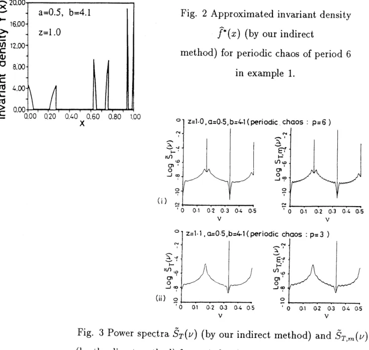
Fig-ures 2 and 3 show $f^{*}(x)$ and the power spectrum $\tilde{S}_{T}(\nu)$ for periodic

chaos of period 6 which are calculated by our $method^{[8],[9]}$_. _{In this}

(9)

that edges of the support of $f^{*}(x)$ will coincide with the partition

points. In the calculation of $\tilde{S}_{T}(\nu)$, thefinite discrete Fourier

trans-form of $\{\rho(k)\}_{k=0}^{T-1}(T=1,024\cross 6)$ is used instead of using Eq.(12).

On the other hand, $S_{T,m}(\nu)$ is obtained by averaging $m=200$

dis-crete Fourier transforms of trajectories of length $T$. The spectrum

$\tilde{S}_{T}(\nu)$ is in good agreement with _{$S_{T,m}(\nu)$} except for fluctuations in

the latter.

Fig. 2 Approximated invariant density

$\hat{f}^{*}(x)$ (by our indirect

method) for periodic chaos of period 6

in example 1.

Fig. 3 Power spectra $\tilde{S}_{T}(\nu)$ (by our indirect

method) and $\tilde{S}_{T,m}(u)$

(10)

Example 2 Let

$\tau(x)=\{\begin{array}{l}x+ux^{z}(x-x_{p})/(1-x_{p})\end{array}$ $0\leq_{p^{X}}\leq_{X^{X_{p}}}x<\leq 1$

where $\tau(x_{p})=1,$

$u>0,1<z<2$

.

This map generates

inter-mittent chaos with the power spectrum $1/f^{\delta}$. Figure 4 shows the

power spectrum $S(\nu)$ by our $method^{[10]}$ (the smooth solid line) and

$S_{T,m}(\nu)$ with $T=2^{15}$ and $m=100$ by the direct method (the

fluc-tuated line), each of which is in good agreement each other in wide

frequency range. In applying our method, we used $s(x)=x^{-(z-1)}$

because $\tau$ has the unbounded invariant density with a $(z-1)$-th

order pole at $x=0$. In this figure, the broken line shows the

Pro-caccia and Schuster’s estimate [11] of the spectrum when $\nu$ goes to

$0$ which does not coincide well with the former two.

屋

$\underline{\infty OO}0$

log(f)

Fig. 4 Comparison of power spectra calculated by using three

(11)

References

[1] S.Ulam, Problems in modern mathematics, Intersience Pub.

(1960).

[2] T.Y.Li, J.Approx. Theo., 17, pp.177-186(1976).

[3] S.Grossmann and S.Thomae, Z. Naturforsch., 32a, $1353- 1363$

(1977).

[4] S.J.Chang and J.Wright, Phys.Rev.A, 23, $1419- 1433$ (1981).

[5] Y.Oono and Y.Takahashi, Progr.Theo.Phys., 63-5, 1804-1807

(1980).

[6] Y.Takahashi and Y.Oono, Progr.Theo.Phys., 71-4, 851-854

(1980).

[7] T.Kohda and K.Murao, Trans. IEICE, J65-A-6, 505-512

(1982).

[8] K.Murao and T.Kohda, Trans. IEICE, J67-A-5, 511-518

(1984).

[9] K.Murao and T.Kohda, Trans. IEICE, J68-A-7, 405-406

(1985).

[10] T.Kohda and K.Murao, Trans. IEICE, E73-6, 793-800 (1990).

[11] I.Procaccia and H.Schuster, Phys.Rev., A, $28- 2,1210- 1212$