The Variety of Spontaneously Generated
1
Tropical Precipitation Patterns found in
2
APE Results
3
Kensuke NAKAJIMA
4
Faculty of Sciences, Kyushu University, Fukuoka, Japan
5
and
6
Yukiko YAMADA
7
Graduate School of Science, Hokkaido University, Sapporo,
8
Japan
9
and
10
Yoshiyuki O. TAKAHASHI
11
Center for Planetary Sciences, Kobe, Japan
12
Kobe University, Kobe, Japan
13
and
14
Masaki ISHIWATARI
1
Faculty of Science, Hokkaido University, Sapporo, Japan
2
and
3
Wataru OHFUCHI
4
Earth Simulator Center, Japan Agency of Marine Science and
5
Technology, Yokohama, Japan
6
and
7
Yoshi-Yuki HAYASHI
8
Center for Planetary Sciences, Kobe, Japan
9
Kobe University, Kobe, Japan
10
August 17, 2012
11
Corresponding author: Kensuke Nakajima, Faculty of Sciences, Kyushu Univer- sity, 6-10-1, Hakozaki, Fukuoka, Fukuoka 812-8581, Japan.
E-mail: [email protected]
Abstract
1
We examine the results of the Aqua-Planet Experiment Project (APE)
2
focusing mainly on the structure of equatorial precipitation in the subset of
3
participating models for which the details of model variables are available.
4
In spite of the unified set-up of the APE, the Hovm¨ellor plots of precipita-
5
tion in the models exhibit wide range of diversity, presumably resulting from
6
the diversity among implementations of various physical processes. Never-
7
theless, the wavenumber-frequency spectra of precipitation exhibit certain
8
degree of similarity; the power spectra can be divided into Kelvin, westward
9
inertio gravity, and “advective” components. The intensity of each of these
10
three components varies significantly among different models. The compos-
11
ite spatial structures corresponding to the above three components are pro-
12
duced by performing regression analysis with space-time filtered data. The
13
composite horizontal structures of the Kelvin and westward inertio gravity
14
components are similar among the models and resemble to those expected
15
from the corresponding equatorial shallow water wave modes. These resem-
16
blances degrade at the altitude levels where the value of phase velocity is
17
near the zonal mean zonal wind speed. The horizontal structures of the
18
“advective” component diverge significantly among models. The composite
19
vertical structures are strongly model dependent for all of the three com-
20
ponents. The comparison among vertical and horizontal structures of con-
21
vective and stratiform heating of the composite disturbances indicates that
1
the diversity of vertical structures originates from the difference in physical
2
processes, especially, the implementation of cumulus parameterization.
3
1. Introduction
1
Convective activity in the earth’s tropical atmosphere is recognized to
2
exhibit a hierarchical structure including individual cumulonimbi, mesoscale
3
features, cloud clusters (Houze and Betts 1981), various kinds of synoptic
4
scale disturbances such as convectively coupled equatorial waves (Kiladis
5
et al. 2009), intraseasonal variability (ISV) (Madden and Julian 1972),
6
and climatological features like the intertropical convergence zone (ITCZ)
7
or the convection centers. Each of the classes in the hierarchy has unique
8
importance in the role, for example, in the maintenance of the climate
9
system (Sherwood et al. 2010), in predictability issues of numerical weather
10
prediction, and in severe meteorological phenomena central to the disaster
11
prevention. Reproduction and understanding of the hierarchy of convective
12
activity is thus one of the most important theme of tropical meteorology.
13
In our efforts to capture the hierarchical structure, there remains a large
14
degree of difficulty. The most obvious difficulty is its extremely wide range
15
of spatial and temporal scales; there is four orders of magnitude difference
16
from the smallest member, individual cumulonimbi having 1–10 km scale,
17
to the largest member, ISV and ITCZ having a global scale. If we wish
18
to simulate whole of the hierarchical structure explicitly, we have to run a
19
global cumulus resolving model; its execution requires huge computational
20
resources (Tao and Moncrieff 2009). Up to present, only a very limited
number of such explicit calculations have been accomplished (Satoh et al.
1
2008). Other than such explicit simulations, any kinds of global models are,
2
more or less, compromised to incorporate the effects of the smaller classes of
3
the hierarchy, i.e., cumulonimbi and mesoscale systems. The most common
4
way of compromise has been to employ cumulus parameterization, although
5
there are a few exceptional attempts to avoid cumulus parameterization by
6
using “distorted” dynamical equations (Kuang et al. 2005).
7
Although it is true that computational resources are rapidly develop-
8
ing, a certain level of cumulus parameterization is considered to remain in
9
global models at least for long term simulations like those for the projection
10
of possible global warming. And hence, the knowledge on the performance
11
of numerical models employing cumulus parameterizations in the reproduc-
12
tion of the tropical convection hierarchy remains important in some unfore-
13
seeable period in the future. At present, there are not small number of
14
cumulus parameterization used in operational or community atmospheric
15
models including adjustment type schemes (Manabe et al. 1965), mass flux
16
type schemes (Tiedtke 1989), and schemes employing ensemble of cumulus
17
(Arakawa and Schubert 1974). In spite that a cumulus parameterization
18
scheme is highly tuned to reproduce the behavior of the real atmosphere
19
when used in an atmospheric model, it has been known that the properties
20
of tropical atmospheric convection represented in numerical models exhibit
21
wide variety among models, and it is still agreed that no single specific
1
parameterization scheme can be nominated as the one that is the most
2
suitable for reproducing the reality. We have to examine how and why
3
various models behave differently by comparing the results with such mod-
4
els in a common setup as an inter comparison project such as Atmospheric
5
Model Intercomparison Project (AMIP) or Coupled Model Intercomparison
6
Project (CMIP).
7
The Aqua-Planet Experiment Project (APE) is an attempt to compare
8
the behavior of modern sophisticated numerical models used for numeri-
9
cal weather prediction or climate simulation in the simplest set-up of the
10
“aqua-planet”, i.e. a virtual planet wholly covered with ocean of fixed sur-
11
face temperature. The context and aim of the APE are fully discussed in
12
Blackburn and Hoskins (2012), where the history and the position of ide-
13
alized AGCMs (atmospheric general circulation model) experiments in the
14
framework of atmospheric research in general are also stated. The setup of
15
aqua-planet was first employed purposefully by Hayashi and Sumi (1986)
16
in order to find the “natural” behavior of tropical atmospheric convection.
17
They succeeded in identifying the hierarchy, or its substitute in low resolu-
18
tion model employing cumulus parameterization, that includes cloud clus-
19
ters, super cloud clusters, ISV, tropical cyclones and double ITCZ. One
20
might regard this setup is trivial or easy one because it is free from com-
21
plex treatment of land surface and associated hydrology and/or vegetation
1
schemes. However, it presents a unique and difficult challenge to AGCMs;
2
being free from the external forcing provided from the inhomogeneity of
3
underlying surface, the model atmosphere have to determine its behavior
4
by itself, and hence both of the strength and the weakness of models are
5
exposed clearly. In fact, as early as at the beginning of 1990’s, it has been
6
clarified that the choice of cumulus parameterization strongly affects several
7
fundamental properties of AGCM such as the behaviors of tropical distur-
8
bances (Numaguti and Hayashi 1991a) or the structure of ITCZ (Numaguti
9
and Hayashi 1991b).
10
The present paper describes the behavior of equatorial precipitation
11
structures in CONTROL experiments conducted in the APE (Neale and
12
Hoskins 2000). Among the series of classes of the hierarchical structure of
13
tropical precipitation convection, we will focus our attention to the “inter-
14
mediate” scale structure, i.e., convectively coupled equatorial waves (Kiladis
15
et al. 2009), because of the following reasons in particular. The first reason,
16
which is the most trivial, is that the smaller classes, i.e., individual cumu-
17
lonimbi and mesoscale systems, are below the resolvable scales of most of
18
the AGCMs participating in the APE. The second reason, which is also
19
trivial, is that the larger classes, i.e., ISV, the convection centers and the
20
ITCZs, are presumably strongly affected by the present idealized, unreal-
21
istic setup of aqua-planet. We should suspect that the behaviors of the
1
models by themselves are unknown. It might be possible that the mecha-
2
nism governing the ISV, if exist, obtained in the present setup is different
3
from that of the ISV in the real atmosphere. The larger scale features
4
should be examined from a wider perspective elsewhere (see, for instance,
5
(Nakajima et al. 2011)). The third reason, which is the most important,
6
is that, as will be shown later, the behaviors of convectively coupled waves
7
in the models in the APE display rich variety possibly depending on the
8
choice of cumulus parameterization employed. The examination of variety
9
of the properties of convectively coupled equatorial waves (CCEWs) in the
10
APE should enhance our knowledge on the underlying mechanism govern-
11
ing the CCEWs in coarse resolution AGCMs, which would lead us to the
12
guiding principles on how to tune cumulus parameterization so as to better
13
represent the behavior of the real atmosphere.
14
Among the CCEWs, we further confine our attention to Kelvin waves,
15
equatorially symmetric westward gravity waves, and disturbances presum-
16
ably advected westward by the background wind. These categories of
17
CCEWs partially overlap with those examined in the wavenumber-frequency
18
spectral analysis of observational data by Wheeler and Kiladis (1999). In
19
other words, we exclude equatorial Rossby waves with especially large lon-
20
gitudinal scales and all of the equatorially asymmetric waves from our at-
21
tention. In these disturbances, divergence is absent or weak at the equator
1
(Yang et al. ,2007a). Consequently, it is expected that they are not strong
2
in the experiments with CONTROL SST, where the distribution of SST has
3
a rather sharp peak at the equator and the ITCZs are mostly confined to
4
the equator (Blackburnet al., 2012a). The properties of these disturbances
5
should be examined elsewhere including the comparative analysis of the ex-
6
periments with the other profiles of SST, two of which have more broad
7
peak profiles.
8
The present paper is organized as follows. Section 2 will explain the
9
setup of experiment. Because details of the APE project are given else-
10
where (Blackburn and Hoskins,2011), only brief summary will be presented.
11
Section 3 will present the methods of analysis. Section 4 will compare gross
12
feature of CCEWs in the APE models. Section 5 will compare the compos-
13
ite structure of three categories of CCEWs produced from the regression
14
analysis of spectrally filtered time series from the several selected models.
15
Discussions and conclusions will be given in the last two sections.
16
2. Setup of Experiments
17
The experiments to be examined in this paper is the CONTROL case
18
of the APE. As for the details not touched here, readers are referred to the
19
context paper (Blackburn and Hoskions 2012) or the original proposal paper
20
(Neale and Hoskins 2000). The SST distribution is zonally uniform and fixed
1
in time. The meridional structure is shown in Fig. 1. The SST profile is
2
characterized with a rather sharp single peak located at the equator and
3
north-south symmetric. The latitudinal gradient is steep from subtropics
4
to midlatitude, whereas it flattens in high latitude region. Reflecting this
5
character, climatological subtropical and mid-latitude jets effectively merge
6
to form a single very strong jet located in subtropics.
7
In the APE archive, the results of 17 AGCM runs from 15 groups are
8
accumulated. A brief summary of the specification of the models is given
9
in Table 1. Among these, 7 groups provided more detailed time series on
10
additional model variables for 8 runs, from which we obtain the composite
11
structures as presented later. It is worth mentioning that even the subgroup
12
for which composite analysis is performed contains a wide variety of spatial
13
resolutions and cumulus parameterizations. More complete specifications
14
are given in the APE-ATLAS (Williamson et al. 2011) to which readers are
15
referred to.
16 Table 1
Fig. 1
3. Methods of analysis
1
3.1 Data
2
The data used in this study are the 6-hourly one year time series (“TR”)
3
of CONTROL experiments and the “additional transient time series” con-
4
taining multilevel model variables of the following seven AGCM runs, AGU-
5
forAPE, CSIRO std, ECMWF05, ECMWF07, GSFC, LASG, and NCAR.
6
In the present paper, we mainly examine the latter data. The former con-
7
tain model variables on very limited model levels, and are only consulted
8
in order to check the representativeness of the seven model runs focused in
9
this study among all of the AGCM runs. The variables we examined are
10
zonal wind, meridional wind, vertical velocity, temperature, geopotential
11
height, specific humidity, and, precipitation flux. In addition, temperature
12
tendency due to parameterized convective process and that due to resolved
13
condensation are used in the composite analysis of disturbances. Note that
14
data for temperature tendency terms of CSIRO std and resolved condensa-
15
tion of LASG are missing.
16
3.2 Hovm¨ ellor plots and wavenumber-frequency spectra
17
In section 4, we show plots of time evolution (“Hovm¨ellor” plots) and
18
wavenumber-frequency spectra of precipitation along the equator. For the
19
models that do not have grid points on the equator, the averaged data of
1
the two grid points nearest to the equator of the both hemispheres are used
2
instead. Wavenumber-frequency spectra are obtained by the following pro-
3
cedures. (i) From the original 1-year time series of each model run, ten time
4
series of the period of 90-days which begin at every 30 days from the begin-
5
ning of the year are extracted. (ii) From each of the 90-day segment, linear
6
trend, which is estimated using least square fit, is subtracted. (iii) Double
7
Fourier transform is executed to obtain wavenumber-frequency spectrum of
8
each of the segments. (iv) All of these wavenumber-frequency spectra of
9
the ten 90-day segments are averaged to obtain the final estimate of the
10
wavenumber-frequency spectrum of precipitation of each model.
11
In addition to the wavenumber-frequency spectra, we present the “en-
12
hanced” power spectra of the meridionally symmetric component of precip-
13
itation within 5 degree latitudes around the equator. The method to obtain
14
the enhanced spectra basically follows that used in Wheeler and Kiladis
15
(1999). (i) Time series of north-south symmetric component of precipita-
16
tion is made for each latitude. (ii) Wavenumber-frequency spectra of this
17
time series is produced in the same way as explained in the previous para-
18
graph. (iii) Thus obtained power spectra for all latitudes within 5 degrees
19
from the equator are averaged. (iv) The averaged spectra are divided by
20
their “background” spectra which are obtained by applying 1-2-1 smoothing
21
40 times in wavenumber and frequency space.
1
3.3 Wave-type filtering
2
In section 5, we examine the structures of precipitation disturbances
3
at the equator distinguishing the types of relevant equatorial disturbances.
4
The method of separation basically follows that in Wheeler et al. (2000).
5
We focus three types of convectively coupled equatorial disturbances; Kelvin
6
(n=-1), westward inertio gravity (n=1), and “advective” components (here-
7
after these three components are referred to as K component, WIG compo-
8
nent, and AD component, respectively). The last one has been referred to as
9
“TD-type” component in Wheeler and Kiladis (1999). In the wavenumber-
10
frequency domain of TD-type component, Yang et al. (2007a) identified
11
equatorial Rossby waves modified by the Doppler effect due to easterly
12
basic flow. However, the ITCZs appearing in the CONTROL experiment
13
in most models are sharply concentrated at the equator (Blackburn et al.
14
2012a), so that the disturbances in the wavenumber-frequency domain cor-
15
responding to TD-type or “Doppler shifted Rossby waves” do not necessarily
16
accompany vorticity. Association of vorticity is an indispensable character
17
of tropical depressions (TD) or Rossby waves. From this reason, we choose
18
the name of “advective component” instead.
19
The procedure for isolating each of the three types of components again
20
basically follows that of Wheeler et al. (2000). (i) We perform double
1
Fourier transformation of the three dimensional time series of the variables
2
to be analyzed in longitude and time. (ii) We adapt the wavenumber-
3
frequency spectral coefficients to those corresponding to the three types of
4
disturbances by passing through the wavenumber frequency domains whose
5
specifications are described below. (iii) We perform inverse double Fourier
6
transformation of the filtered wavenumber frequency coefficients to obtain
7
the three dimensional time series of variables representing each of the three
8
types of disturbances. The definitions of the filters for the three disturbance
9
types are shown in Fig. 2.
10
The range of equivalent depth associated with the filter for K compo-
11
nent is broader than that in Wheeler and Kiladis (1999) where the range
12
between 8m and 50m is employed. By the present choice, we intend to cover
13
the wide variety of signals along around the Kelvin wave dispersion curves
14
appearing in the various APE runs. In each of the APE runs, however, the
15
range of the equivalent depth of its dominant K component is much nar-
16
rower, as will be presented later. The domain of AD component is chosen
17
considering following constraints. First, the lower bound of the westward
18
propagating zonal wavenumber is selected to be four so as to avoid possible
19
“contamination” by the disturbances of the type of planetary scale Rossby
20
waves. Second, the upper bound of the frequency is set be 0.5 d−1 so as
21
to avoid the overlap with WIG component. Third, the lower and upper
1
bounds of characteristic velocity are selected to be 2.5 m/s and 12 m/s,
2
respectively, so as to cover wide variety of possible disturbances that will
3
fall in the category of “advective component” appearing in the various APE
4
runs. The domain for WIG component follows that used in Wheeler and
5
Kiladis (1999).
6
3.4 Composite structure
7
In Section 5, we present composite structure of K, WIG, and AD com-
8
ponents along equator appearing in each of the seven AGCM runs. The
9
composite structure is obtained by performing (simultaneous) regression
10
analysis of the time series of model variables filtered through one of K,
11
WIG or AD filters described in the previous subsection. Thanks to the
12
idealized zonally symmetric configuration of the CONTROL experiment of
13
the APE, the procedure of regression is quite simple. We extract a time
14
series of a filtered model variable (predictand) at a height and a latitude,
15
and shift the extracted data longitudinally by a certain zonal length, and
16
calculate the slope of linear regression of the shifted time-longitude data
17
against filtered precipitation at the equator. By repeating this procedure
18
for all latitudes, heights, and zonal shift lengths, we can obtain the com-
19
posite three-dimensional structure of the model variable for the disturbance
20
of the filter used. We will not perform the lagged regression analysis, but
1
averaged temporal evolution of traveling disturbances is, to some extent,
2
expected to be captured as the zonal structure of the simultaneous compos-
3
ite. The details of the temporal evolution may be of interest, but it is left
4
for future research.
5
It should be borne in mind that the magnitude of the regression slope
6
of a particular variable at certain position for a particular model does not
7
necessarily represent the intensity of the model variable actually realized in
8
the model; it depends on the intensity of the filtered rain rate along the
9
equator realized in the model, which varies significantly on different models
10
as will be shown shortly below. The units of the regression slope are the
11
units of the predictand per unit rain rate. However, for convenience, we
12
multiply the values of the regression slope by a normalization intensity of
13
precipitation, which is 0.0001 [kg·s−1·m−2], and represent all predictand
14
with their original units.
15 Fig. 2
4. Behavior of equatorial precipitation in the APE
1
models
2
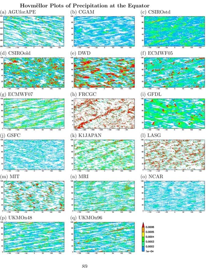
4.1 Hovm¨ ellor plots of equatorial precipitation
3 Fig. 3
Fig. 4 Fig. 5 Temporal evolution of precipitation at the equator of each model is
4
shown in Fig. 3, where one can find quite a wide variety of representations
5
of the hierarchical structure of equatorial precipitation among the different
6
models. The calculated equatorial precipitation features seem to depend on
7
both of the physical processes and the spatial resolution. For example, the
8
higher resolution models such as DWD, ECMWF, FRCGC, CSIRO exhibit
9
fine spatial structures, which cannot be observed in the lower resolution
10
models, such as AGUforAPE, CGAM etc. The results of ECMWF 05 and
11
ECMWF 07 are interesting. They have the same resolution but slightly
12
different cumulus parameterizations, and show considerably different be-
13
haviors. The variety exemplified by the APE models is so widespread that
14
it is difficult to describe meaningfully how the behavior of one model differs
15
from that of another. So we only point out several noteworthy features.
16
In some models, eastward propagating planetary scale signals, whose
17
propagation speeds are not very different from that of ISV in the real atmo-
18
sphere (Madden and Julian 1994), are notable but with different intensity.
19
FRCGC, i.e., NICAM run shows the most prominent eastward propagating
20
signal as was described in Miura et al. (2005) and Nasuno et al. (2008).
1
It is also evident in the results of K1Japan, two versions of UKMO, and
2
two versions of ECMWF, but the intensity or detailed structures differ con-
3
siderably. On the other hand, such eastward propagating low wavenumber
4
signal is weak or absent in AGUforAPE, NCAR, and CISRO-old. In spite
5
that these models are common in lacking notable eastward propagating sig-
6
nal, they differ significantly; precipitation in NCAR is generally weak and
7
rather uniform, whereas that in CISRO-old is generally intense, and that in
8
AGUforAPE is organized in westward propagating structures.
9
If we focus on smaller scale features, precipitation occurs near the “grid
10
scale”, i.e. nearly the smallest scale resolvable in all models in general.
11
However, the behavior of grid scale precipitation varies significantly. The
12
life time of such grid-scale precipitation varies among models ranging from
13
about one day to nearly ten days. Moreover, the direction of migration of
14
those grid scale precipitation structures also differ among models; those in
15
AGUforAPE and MIT move generally westward, those in ECMWF05 and
16
GFDL are nearly stationary, and those in UKMO, K1JAPAN, ECMWF07,
17
DWD, and CSIRO move generally eastward.
18
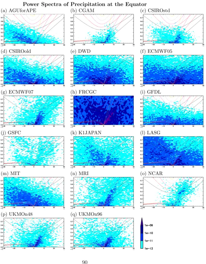
4.2 Wavenumber-frequency spectra of precipitation
1
In contrast to the extremely rich variety in the appearance of equato-
2
rial precipitation in longitude time plot, the wavenumber-frequency spectra
3
of the equatorial precipitation of 17 model runs (Fig. 4) exhibit some de-
4
gree of similarity. The most common feature is the eastward propagating
5
signal. In most models, the dominant power of the eastward propagating
6
signals is distributed mainly along respective dispersion relation of equa-
7
torial Kelvin wave mode, although the intensity, characteristic equivalent
8
depth, and dominant zonal wavenumber differ among the models. The iden-
9
tification of these signals as the equatorial Kelvin wave type is supported
10
by the composite analysis of its spatial structure, which will be shown later.
11
The eastward propagating signal in NCAR is, however, somewhat differ-
12
ent from those in other models; the dominant wavenumber, 5–10, is much
13
larger than those in other models, 1–5. Moreover, the strong power seems
14
to be distributed along the dispersion curve of n=1 eastward inertio grav-
15
ity wave mode . Strangely, the wavenumber-frequency spectrum of mid-
16
tropospheric vertical velocity (not shown) exhibits much weaker wavenum-
17
ber dependence, so that the ratio of the intensity of precipitation to the
18
intensity of vertical velocity, which might be interpreted as the gross sensi-
19
tivity of the response of the latent heating to the grid scale ascent, strongly
20
depends on wavenumber; precipitation is much more sensitive to vertical
21
velocity in zonal wavenumber 5–10 than in zonal wavenumber 1–5. In the
1
results of other models, there are not such distinct variation of sensitivity,
2
and their magnitudes are more or less similar to that for the signal around
3
wavenumber 5–10 of NCAR. It should be also noted that the reduced sensi-
4
tivity of precipitation to vertical velocity in NCAR is observed only near the
5
equator. This latitudinal dependence may be related to the latitudinal pro-
6
file of ITCZ; NCAR is characterized with distinct “double ITCZ” structure,
7
but most of other models in the APE are characterized with “single ITCZ”
8
for the CONTROL SST profile. These evidences suggest that the eastward
9
propagating signals in NCAR bear some character of eastward propagating
10
inertio gravity wave with equivalent depth of about 12 m. However, as will
11
be shown later, its composite structure is not very different from that of
12
equatorial Kelvin wave.
13
In contrast to more or less common emergence of Kelvin wave type sig-
14
nals, the intensity and the spreading of “background component” vary much
15
more drastically among the models. They reflect both the climatological
16
structure of ITCZ and the structure of precipitation events. As is described
17
in Blackburnet al. (2012a), the mean precipitation intensity at the equator
18
varies over a factor of 3 among the models, and, as will be shown in the
19
next section, the models with the larger mean precipitation intensity exhibit
20
the larger power of over-all variance of precipitation. The wavenumber and
21
frequency bandwidths are, from the definition of Fourier components, re-
1
lated to the degree of concentration of precipitation in the real space. More
2
widespread background component found in DWD, ECMWF05, LASG, and
3
FRCGC reflect more concentrated grid-scale precipitation structures as is
4
recognized in Fig. 3.
5
It is interesting that, in most models, westward component extends to
6
the higher frequency than eastward component does. Yang et al. (2009)
7
indicate that similar feature of wavenumber-frequency spectrum of precip-
8
itation is found in Hadley center models and the observation of real atmo-
9
sphere. The Doppler effect due to low level background easterly wind may
10
be the origin of the east–west asymmetry, but further study is required to
11
clarify the issue.
12
Intricate features can be seen more clearly in Fig. 5, where the sig-
13
nal enhancing technique of Wheeler and Kiladis (1999) is employed on
14
those wavenumber-frequency spectra. The westward propagating back-
15
ground component are divided into two components. One is called, fol-
16
lowing the notation of Wheeler and Kiladis (1999) used for observed OLR
17
(outgoing longwave radiation), “inertio gravity wave’, or WIG, component
18
whose signals are found in the region along dispersion curves of westward
19
inertio gravity waves. The other is called “advective” (AD) component in
20
this paper because they are generally distributed around straight lines pass-
21
ing through the origin in the wavenumber-frequency space, which indicates
1
that disturbances are advected by background easterly winds. However,
2
the actual relationship between the propagation speed of AD component
3
and mean zonal wind is not straight forward as will be discussed in Section
4
6.1(c).
5
The behaviors of WIG components exhibit significant variety among
6
models, although to a smaller degree than for those of AD components.
7
In AGUforAPE and CGAM, the WIG signal is very weak, while it is dis-
8
tinct in LASG and K1JAPAN. In GSFC, the WIG signal is apparent in
9
the enhanced power spectrum (Fig.5(j)), although the absolute intensity is
10
not large (Fig.4(j)). Note that not only the intensity but also the distribu-
11
tion varies over the wavenumber-frequency space; the signals cover a wide
12
range of wavenumber in LASG (Fig.4(l)) and K1JAPAN (Fig.4(k)), while
13
the higher wavenumber signals can be noted in GSFC (Fig.4(j)). It is also
14
worth noting that there is a gradual change of the characteristic equiva-
15
lent depth of WIG component as wavenumber varies; WIG component of
16
the larger scale tend to have the shallower equivalent depth. The most
17
clear example is LASG (Fig.5(l)). This tendency suggests that the strength
18
of coupling between convective heating and large scale convergence asso-
19
ciated with WIG component might depend on the characteristic period of
20
disturbances and result in the varying degree of “reduced stability” effect
21
discussed by Gill (1982).
1
Because of the idealistic and clean setup of the APE project, one can
2
easily recognize several types of planetary scale disturbances other than the
3
convectively coupled equatorial waves and advective signals. One is the
4
quasi-stationary wavenumber five signal. Most prominent example can be
5
found in the result of NCAR (Fig4(o), Fig5(o)). Together with the ten-
6
day period wavenumber six component nearby, it seems to be associated
7
with the midlatitude baroclinically unstable waves like those examined by
8
Zappa et al. (2011). Another example is the clear appearance of diurnal
9
and semi-diurnal migrating tides (Woolnough et al. 2004). Additionally, we
10
can find several types of normal mode waves which include the counterparts
11
of those observed in the real atmosphere such as the 33-h Kelvin wave of
12
Matthews and Madden (2000) and the n = 0 mixed-Rossby gravity mode
13
and then >1 Rossby modes of Hendon and Wheeler (2008). These features
14
are only marginally identifiable in the wavenumber-frequency spectra of
15
precipitation, but are more easily confirmed in the spectra of zonal wind or
16
surface pressure (not shown here). Among these waves, the representation
17
of the 33-h Kelvin wave is found to be sensitive to the vertical resolution
18
and/or the upper boundary conditions of the model, whereas that of other
19
types of planetary scale disturbances mentioned above is less sensitive. The
20
description of those waves is left for future research.
21
In many of the experiments, tidal signals significantly modulate the sig-
1
nals of tropical precipitation associated with the Kelvin or AD component
2
significantly. Such modulation results in high frequency, low wavenumber
3
component that sometimes overlaps the wavenumber-frequency domain of
4
WIG and/or the region of eastward inertio gravity wave modes. Most clear
5
example that the modulation of K component can be observed is that of
6
UKMO (fig. 5(p,q)); the signals going through (wavenumber, frequency)
7
= (−5,0.9) and (−10,0.6) in the wavenumber-frequency domain of WIG
8
component are the projection images of the modulation of those for K com-
9
ponent.
10
5. Spectral filtering analysis
11
As described in the previous section, there is a prominent variety in
12
the space-time structures of equatorial precipitation calculated by the APE
13
models. It it highly probable that various different choices of discretiza-
14
tion schemes, spatial resolution, and implementations of physical processes
15
among the models result in the variety of model behavior. However, it is a
16
quite difficult task to point out one or more items that may cause one or
17
more particular differences in such structures. Before any progress be made,
18
it is necessary, at least, to describe the circulation structures associated with
19
the characteristic space-time structures of equatorial precipitation, and dif-
ferences among them.
1
As an attempt to describe systematically the various behaviors of equa-
2
torial precipitation in the APE models, we decompose the time series data
3
of variables produced by each model into the contributions of Kelvin, WIG,
4
and AD components, construct composite structures of them, and com-
5
pare the characteristics of composite disturbances. The experiments to be
6
analyzed are the subset CONTROL runs, where detailed transient data
7
are additionally submitted. They are AGUforAPE, CSIRO, ECMWF05,
8
ECMWF07, GSFC, LASG, and NCAR. Although the spectral property of
9
each component differs among models, we use the same definition of the
10
filters for each model. As a result, some of the dominant spectral power are
11
excluded from the composite for some models; most suffering from this is
12
WIG component in LASG where the contribution from the low wavenumber
13
region is out of the range. However, by this choice of the filters, we prioritize
14
the uniform application of filters to the results of all of the models to be
15
compared over the completeness of coverage of the three spectral compo-
16
nents appearing in the results of each model. The wavenumber-frequency
17
domains of three kinds of filters are shown in Fig. 2.
18
5.1 Intensities of Kelvin, WIG and AD components
1 Fig. 6
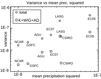
Fig. 7 Before examining the spatial structure of each component, we compare
2
the intensities of three components of the additionally contributed seven
3
APE models. Fig. 6 shows the variance of equatorial precipitation calculated
4
from the time series with K, WIG, and AD filters; the absolute values
5
(Fig. 6(a)) and the values normalized by the variances of original, unfiltered
6
time series of precipitation of corresponding models (Fig. 6(b)). Fig. 7
7
is a scatter plot showing the relationship between the mean precipitation
8
squared and the two kinds of precipitation variances; shown by circle is the
9
total variance, i.e., the variance of the original time series of each model, and
10
shown by square is the sum of the variances of the three filtered components.
11
It is evident from Fig. 6(a) that the intensities of all components are strongly
12
model dependent. LASG and ECMWF05 are members that exhibit most
13
intense disturbances, whereas NCAR, GSFC, and CSIRO are those with
14
weakest. As for the intensity sum of K, WIG, and AD components, that
15
of ECMWF05 is about 30 times as large as that of NCAR. (see also those
16
plotted by squares in Fig. 7).
17
In Fig. 6(b), we can point out two aspects commonly noted among the
18
models. First, the sum of the three components contributes to roughly
19
about ten percents of the total variance of precipitation of each model.
20
the contribution other than those three components is not at all negligi-
21
ble. Second, WIG component is weakest in the three kinds of disturbances.
1
However, the relative intensity of variances between K component and AD
2
component varies largely among the models. There is a weak negative cor-
3
relation between the intensities of K and AD components. AGUforAPE and
4
ECMWF07 show contrasting features; AD component dominates in AGU-
5
forAPE, whereas K component dominates in ECMWF07. It is an important
6
issue to understand how the magnitudes of contributions of these three com-
7
ponents to the total variance of precipitation are determined. However, it
8
is left for future studies.
9
It may be worth mentioning that both the unfiltered total variance and
10
the variance sum of the three components are well correlated with the aver-
11
age precipitation intensity (Fig. 7). Total variance, for instance, is propor-
12
tional to the cube of the average precipitation rate. LASG and CSIRO are
13
outliers exhibiting the larger and the smaller variance expected from the
14
tendency shared by the models, respectively. The variety of total variance
15
corresponds to the variety of the probability distribution function (PDF)
16
of precipitation. As shown in Fig.18 of Blackburn et al. (2012a), in the
17
models with the larger variance, EC05 and LASG, the PDFs have long tails
18
in the strong precipitation compared with the PDFs in the models with
19
the smaller variances, e.g., NCAR, GSFC, or CSIRO. One may imagine
20
that variance is the larger in the models with the higher spatial resolution.
21
However, it is not true; LASG, in which the total variance is very large,
1
is one of the models with the lowest horizontal resolution, and, EC05 and
2
EC07 differ drastically in the total precipitation variance in spite of their
3
identical horizontal resolution. The PDF of CSIRO does not have a long
4
tail, although its mean precipitation rate is not small. It is more plausible
5
that the variance is more strongly governed by cumulus parameterization.
6
This issue is also left for future research.
7
5.2 Composite structure of Convectively Coupled Equatorial
8
Waves
9
Hereafter, the composite structures associated with K, WIG, and AD
10
components of the seven APE models are examined. As was written in
11
section 3, the composite structures are derived from the regression of corre-
12
sponding filtered variables to the symmetric component of filtered precip-
13
itation intensity at the equator. The variables in the following figures are
14
scaled for 0.0001[Kg/s m2] precipitation anomaly at the reference latitude,
15
180 degree longitude. Note that the intensities of composite disturbances
16
presented in the following figures do not represent the intensities of those
17
disturbances emerging in the models; only their structures matter.
18
a. Composite structure for K component
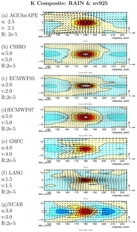
1 Fig. 8
Fig. 9 Fig. 10 Fig. 11 Fig. 12 Fig. 13 Fig. 14 The composite structures for K component are presented in Fig. 8–14.
2
Fig. 8 shows the horizontal structures of precipitation and horizontal wind
3
at the height of 925hPa. In all models, precipitation anomalies are well con-
4
fined near the equator. However, the latitudinal extents somewhat differ;
5
in ECMWF05 and LASG, they are sharply confined around the equator
6
whereas in AGUforAPE, ECMWF07, and NCAR, they are broad. Gener-
7
ally, the north-south extent corresponds to the width of the ITCZ in each
8
model (Blackburn et al. 2012a). The longitudinal structures also differ
9
among the models; in LASG and ECMWF05 and GSFC, they are confined
10
around the precipitation peak, while in AGUforAPE and ECMWF07, they
11
are broader. In NCAR, precipitation anomaly has a wave-like variation
12
with the wavelength of about 6000km, and associated with off-equatorial
13
signal which is delayed with 10 degrees. Similar off-equatorial signal can
14
be found also in GSFC. Note that both of the two models are characterized
15
with distinct double ITCZ structure (Williamson et al. 2011). The hori-
16
zontal wind structures deviate from that expected from the shallow water
17
Kelvin wave (Matsuno 1966); the magnitudes of meridional flows are not
18
very different from those of zonal flows. Convergence of meridional wind
19
commonly occurs at almost the same location as that of zonal wind. Among
20
the seven runs, AGUforAPE exhibits a most deviated horizontal wind struc-
21
ture. Generally, low level horizontal wind driven by condensation heating
1
tends to be confined around the condensation heating (precipitation) area,
2
as is typically indicated by CSIRO, ECMWF05, ECMWF07, and LASG
3
(Fig. 8(b), (c), (d), (f)). However, AGUforAPE (Fig. 8(a)) shows wide
4
spread wind response especially to the west of condensation heating. We
5
can recognize anticyclonic circulations which seem to extend beyond the
6
range of the figure to the subtropical latitudes.
7
Fig. 9 shows the horizontal structures of geopotential and horizontal
8
wind at the height of 850hPa. The horizontal structures of most models are
9
similar to that of shallow water equatorial Kelvin wave (Matsuno 1966) in
10
the sense that zonal component dominates in the wind field and geopotential
11
height and zonal wind are positively correlated and confined around the
12
equator. Wind convergence appears near the precipitation maximum in
13
all of the models. However, precise location of convergence varies among
14
models; it resides 5-10 degrees to the east of the the rainfall maxima in
15
AGUforAPE, CSIRO, ECMWF05 and ECMWF07, about 2 degrees to the
16
east in GSFC and LASG, and about 2 degrees to the west in NCAR.
17
One of the features at the level of 850hPa that deviate from the structure
18
of Kelvin wave, we can recognize significant meridional wind perturbation
19
near the precipitation maximum for all models. It may be worth mentioning
20
that the strength of meridional wind perturbation depends on the choice
21
of variable for the key of regression; the composite horizontal structure
1
based on the regression to low level zonal wind at the equator (not shown
2
here) exhibits much weaker meridional wind, displaying the larger degree of
3
similarity to a shallow water Kelvin wave.
4
The structure of AGUforAPE (Fig. 9(a)) exemplifies a peculiar struc-
5
ture of deviation from that of Kelvin wave. Its zonal wind perturbation is
6
strongly confined in the vicinity of the equator compared to that of geopo-
7
tential height. The meridional wind perturbation, on the other hand, seems
8
to originate in the higher latitudes in the same way as observed at the sur-
9
face level (Fig. 8(a)). By inspecting Fig. 9 and also Fig. 8 more carefully, we
10
can point out that NCAR also show somewhat peculiar features. First, the
11
longitudinal extent of the composite structure is small compared to others;
12
the others show one pair of high and low pressure anomalies along the equa-
13
tor while NCAR shows one and half. This feature is also confirmed in the
14
power spectra of equatorial precipitation (Fig. 4); signals with wavenumber
15
5–10 are dominant in NCAR, whereas those with the smaller wavenum-
16
ber are dominant in the other models. Second, the precipitation anomaly
17
exhibits a significant meridional phase difference; the longitude of maxi-
18
mum precipitation at the latitude of the ITCZ is located at about 10 degree
19
to the west of that at the equator. This horseshoe like structure can be
20
constructed as a superposition of the horizontal structures associated with
21
equatorial Kelvin wave and eastward inertio gravity wave, the latter being
1
shifted by about 5 degrees to the east of the former. Coexistence of those
2
two types of wave structures is consistent with the dominant precipitation
3
signals in the wavenumber-frequency space (Fig. 4(o) and Fig. 5(o)), where
4
intense power appears along the dispersion relation of not only Kelvin wave
5
but also eastward inertio gravity wave having the equivalent depth of about
6
10 m, Also observed is that the horizontal wind structure at the surface level
7
shown in (Fig. 8(g)) resemble that of eastward propagating inertio gravity
8
wave. The composite horizontal structure of K component in NCAR seems
9
to include both of the features of eastward propagating inertio gravity waves
10
and Kelvin waves.
11
In contrast to the resemblance among the models observed in the surface
12
and the lower troposphere, there is considerable model dependence in the
13
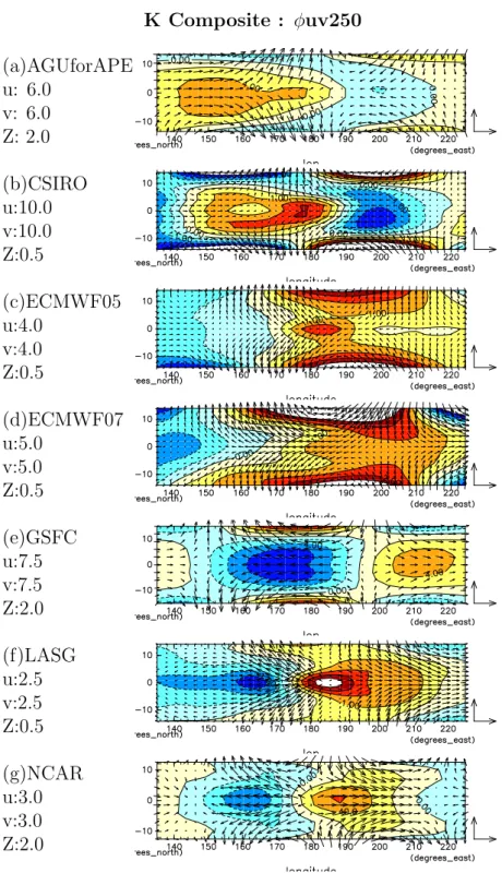
upper tropospheric structures. Fig. 10 shows the horizontal structures of
14
geopotential and horizontal wind at the level of 250hPa for K component.
15
The divergence of zonal wind perturbation around the maximum of precip-
16
itation that is the feature expected for the so called first baroclinic thermal
17
response of Kelvin wave type without background wind is found only for
18
LASG and NCAR. In ECMWF07 and GSFC, the areas of zonal wind di-
19
vergence are found as far as 1500–2000 km to the east of the precipitation
20
maximum. In AGUforAPE, CSIRO, and, ECMWF05, zonal winds are con-
21
vergent at the precipitation maxima; the horizontal divergence that is re-
1
quired as the continuation of the upward flow at the precipitation maximum
2
is accounted exclusively by the divergence of meridional flow. Additionally,
3
significant vortical perturbations are notable in the subtropics, although the
4
phase of the vortice relative to the location of the precipitation maximum
5
varies among the models.
6
The diversity in the upper troposphere appears because the phase ve-
7
locities of the signals of K component, which are typically 10∼30 m/s, are
8
not very different from the zonal mean zonal wind in the upper troposphere
9
in the tropical and subtropical regions in the models. There are mainly two
10
effects caused by the existence of background westerly wind. One is that
11
intensity of thermal response of Rossby wave type changes greatly accord-
12
ing to the intensity of background westerly. The other is that the effective
13
value of equatorialβ including the background wind term−uyy tends to de-
14
crease, since the background westerly tend to reach zero potential vorticity
15
field around the equator (Sardeshmukh and Hoskins 1988). The response
16
structure could be quite sensitive to the subtle difference of the structure of
17
basic wind and heating at the precipitation anomaly. The structure of the
18
vortical perturbation associated with K component in the different models
19
are presented in Appendix for interested readers.
20
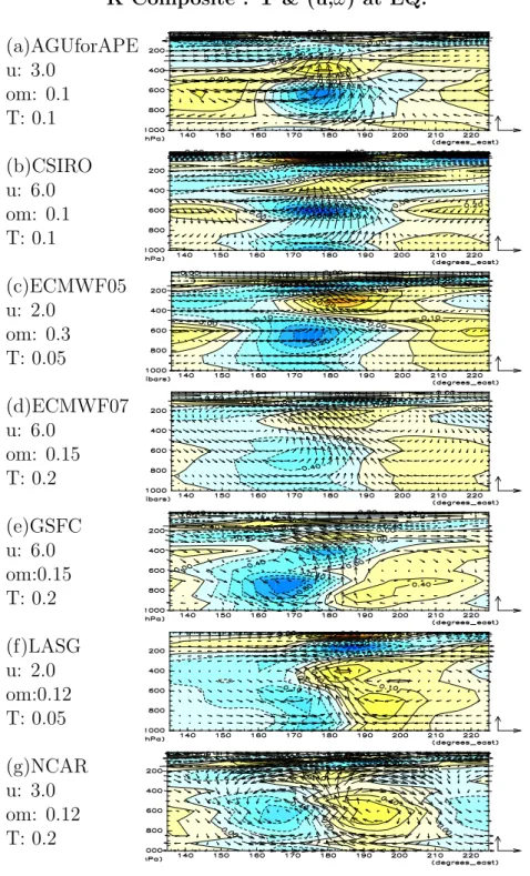
Fig. 11 shows the vertical structures of temperature, zonal wind, and
21
vertical velocity along the equator for K component. We note that temper-
1
ature and vertical velocity anomalies in ECMWF05, ECMWF07, LASG,
2
and NCAR, have westward phase tilt being consistent with wave-CISK the-
3
ory. At the same time, we should emphasize that the vertical structure of
4
temperature anomaly displays a wide variety among the models. We can
5
notice at least four types of temperature perturbations among the models;
6
a signal of the first baroclinic mode extending whole depth of the tropo-
7
sphere, a signal of the second baroclinic mode which has two maxima of
8
amplitude in the troposphere with longitudinal phase shift to each other, a
9
thin signal at around 600hPa that is associated with the melting of ice phase
10
hydrometeor, and another thin signal near the surface possibly associated
11
with the evaporation of raindrops. In each of the models, the four types
12
of temperature signal appear in different combination, intensity, and phase
13
relationship, resulting in the wide variety of the temperature structure.
14
Fig. 12 shows the vertical structures of specific humidity, zonal wind,
15
and vertical velocity along the equator for K component. As a common
16
feature in most models, the humidity field is characterized with a “slant”
17
structure; lower troposphere is moist to the east of the rainfall anomaly,
18
and dry to the west, whereas middle and upper troposphere is dry to the
19
east and moist to the west. In GSFC, however, the longitudinal distribution
20
of humidity anomaly in the lower troposphere around 700–925hPa has the
21
opposite sign to those in the other models; humidity of GSFC is dryer
1
(more moist) to the east (west) of the rainfall anomaly. Another common
2
feature is the existence of a shallow dry region near the surface to the west
3
of the precipitation anomaly, which could be a result of downdraft driven
4
by the cooling associated with, presumably parameterized, evaporation of
5
raindrops.
6
The vertical structures of circulation at the equator shown in Fig. 11
7
and Fig. 12 vary considerably among the models. In the majority of the
8
models, the first baroclinic mode structure dominates in the vertical ve-
9
locity fields, although the location of upward motion does not necessarily
10
corresponds to the area of upper level zonal wind divergence because of
11
the significant contribution of meridional wind divergence mentioned above
12
and also shown later. In most models, the contribution of the second baro-
13
clinic mode structure can be noted by the existence of the westward phase
14
tilt. Examples are found in ECMWF05, ECMWF07, LASG, and NCAR.
15
The composite disturbance of GSFC has one notable feature; a significant
16
downward flow of cool air is found in the lower troposphere to the west
17
of the maximum of precipitation. This is a structure somewhat similar to
18
the mesoscale downward flow that develops below anvil clouds of mesoscale
19
precipitation features (Houze and Betts 1981). However, the zonal extent
20
in Fig. 12(f) is too broad to be regarded as mesoscale; this feature could be
21
explained as a cumulative effect of more compact cold downdrafts found in
1
AD component, which will be presented later.
2
The composite structures of temperature tendency due to parameterized
3
convection (referred to as DT CONV hereafter) and those due to resolved
4
clouds (referred to as DT CLD hereafter) at the equator of K component
5
are shown in Fig. 13 and Fig. 14, respectively. In all models, DT CONV is
6
zonally well confined. In NCAR, regions of significant negative values are
7
observed to the west and to the east of the center of precipitation anomaly.
8
However, recalling that precipitation itself has a zonally wavy structure
9
(Fig. 8(g)), they directly correspond to in situ precipitation anomaly. On
10
the other hand, the vertical structure of DT CONV is strongly model de-
11
pendent. In LASG, it is distributed mainly in the lower troposphere. In
12
AGUforAPE, ECMWF05, and, ECMWF07, the distributions of DT CONV
13
are mostly confined above the freezing levels, whereas those in GSFC and
14
NCAR, they have deep structures extending to both of the lower and the
15
upper tropospheres. In ECMWF07, there is a region of cooling near the
16
surface, presumably resulting from rain evaporation.
17
The distributions of DT CLD are strongly model dependent, not only in
18
their vertical structures but also in their zonal structures. In AGUforAPE
19
and ECMWF05, DT CLD is zonally confined and the vertical structures are
20
similar to those of corresponding DT CONVs. In ECMWF07, GSFC, and
21
presumably NCAR, the distributions of DT CLD spread much more exten-
1
sively in the zonal direction than those of precipitation. In ECMWF07 and
2
GSFC, the distributions are characterized by the second baroclinic mode
3
structure; in the lower troposphere, heating is positive to the east of the
4
center of precipitation anomaly, and negative to the west nicely represent-
5
ing the cooling due to evaporation of stratiform precipitation. It should
6
be noted that the cooling area extends about 3000 km to the west of the
7
center of precipitation anomaly, which is much wider than the typical ex-
8
tent of “mesoscale precipitation features” (Houze and Betts 1981). As a
9
result, overall structure of the heating is somewhat similar to “giant squall
10
lines” observed in the upward motion area of Madden Julian Oscillation
11
as described e.g. in Mapes et al. (2006). There are also shallow regions
12
of cooling near the surface in ECMWF05, ECMWF07 and NCAR. Such
13
cooling near the surface is absent in AGUforAPE.
14
In summary, the composite structures of K component have some degree
15
of similarity to those of the equatorial Kelvin wave mode. This is especially
16
true for the horizontal structure in the lower troposphere. The vertical
17
structures, on the other hand, are shown to be strongly model dependent.
18
It seems that the intensity of disturbances of K component in a particular
19
model seems to increase as the increase of the similarity of the composite
20
structure to the structure of the unstable wave-CISK mode. This point will
21
![Fig. 1. Meridional distribution of sea surface temperature [K] in CONTROL experiment.](https://thumb-ap.123doks.com/thumbv2/123deta/11596206.0/89.892.223.564.409.636/fig-meridional-distribution-sea-surface-temperature-control-experiment.webp)

![Fig. 6. (a) Variance of precipitation along equator for K, WIG, and AD components. Unit is [(kg/m 2 s) 2 ]](https://thumb-ap.123doks.com/thumbv2/123deta/11596206.0/94.892.163.631.281.737/fig-variance-precipitation-equator-wig-ad-components-unit.webp)