Abstract
As large-scale eastward-propagating(EP)precipita-tion systems(PSs)symmetric about the equator, two disturbances are observed; super clusters(SCs)with a horizontal scale of O(1000 km)and a speed of about 15 - 25 ms-1 and the Madden Julian Oscillation(MJO)with a horizontal scale of O(~5000 km)and a speed less than 10 ms-1(Wheeler and Kiladis 1999). When positive-only wave conditional instability of the second kind(POWC) is applied, splitting disturbances in the longitudinal direction first appear in the top-heavy heating case, and then become EP SC-like ones(Yoshizaki, 1991a, Yoshizaki et al. 2012b). As long as idealistic models are used in simplified basic fields, however, splitting distur-bances are attained only in the ‘unusual’ top-heavy heating. Then, a present study is investigated how to get splitting disturbances in the ‘usual’ top-heavy heat-ing.
In the Part 1, the outputs of a dry model with the POWC are compared with those of the non-hydrostatic icosahedral atmosphere model(NICAM)aqua-planet simulation. Using a full model having the same vertical grid structure and basic fields as the NICAM, it is con-firmed that an EP disturbance, whose horizontal struc-ture indicates an asymmetric east-west strucstruc-ture similar to the Gill(1980)response pattern, is attained and the EP speed is comparable to that of NICAM out-puts. Simplification from the full model is pursued by eliminating the nonlinear terms and basic zonal wind and modifying the basic fields of a speed of sound
waves and static stability. It is found that splitting dis-turbances drastically changed into a slowly westward-propagating one when the static stability becomes uniform, which originally has a wavy structure in the troposphere with large(small)values in the lower (upper)layers. It is shown that the variable static sta-bility helps to enhance the top-heavy heating mainly due to the vertical advection of the potential tempera-ture in the heat equation. From these results, it is antic-ipated that the splitting disturbances are obtained in the ‘usual’ top-heavy heating by adopting the realistic static stability.
1. Introduction
In the tropics, several organized structures of large-scale precipitation systems(PSs)are frequently observed with specific horizontal and time scales, such as the Madden-Julian Oscillation(MJO)(e.g., Madden and Julian 1971, Wheeler and Kiladis 1999), super clus-ters(SCs)(e.g., Wheeler and Kiladis 1999), typhoons and hurricanes. Hayashi and Sumi(1986)found SCs using an atmospheric global circulation model in an listic environment of zonally uniform sea surface tem-perature(SST)(aqua-planet). Using satellite data, Nakazawa(1988)showed a multi-scale structure(MSS) of PSs, in which eastward-propagating(EP)PSs coexist with westward-propagating(WP)ordinary cloud clus-ters with a horizontal scale of O(100 km). In most cases(e.g., Nakazawa 1988), SCs interrelate with intra-seasonal tropical variability, such as MJOs, with time
Comparison of Models Having Positive-only Wave CISK with
the NICAM Outputs about Eastward Propagation of
Super Clusters in the Equatorial Region
―Part 1. Approach from a Full Model―
YOSHIZAKI Masanori
*キーワード:positive-only wave CISK, super clusters, eastward propagation, equatorial β
scales of 30-60 days and a horizontal scale of O (~5,000 km). A slow eastward speed is unusual when compared with that of the dry Kelvin wave anticipated from lin-ear theory(e.g., Takayabu 1994; Wheeler and Kiladis 1999). Takayabu(1994)showed a very shallow equiva-lent depth of 15-30 m from cloud disturbances utilizing 3-hourly geostationary meteorological satellite infrared data.
To explain these characteristic features of SCs, although some treated MJOs, many theoretical and numerical studies have been conducted, such as Kelvin-Rossby coupled-type structure(Hayashi and Sumi 1986), the wave conditional instability of the second kind (CISK)theory(e.g., Takahashi 1987), the moist Kelvin
wave theory with positive-only wave CISK(POWC) (e.g., Lau and Peng 1987), the evaporation-wind feed-back(e.g., Neelin et al. 1987), the selective amplification between EP and WP disturbances(e.g., Yoshizaki 1991a), the wind-induced surface heat exchange(Yano et al., 1995), the frictional-convergence feedback(e.g., Wang and Li 1994; Wang 2005), the convectively cou-pled equatorial waves(CCEWs)(e.g., Nasuno et al. 2007, 2008), the extended ones with model-coupled parame-terization of the quasi-equilibrium scheme(Mapes 2000; Majda and Shefter 2001; Majda et al. 2004; Khouider and Majda 2006), the gross moisture stability(e.g., Ray-mond et al. 2009)and so on.
Recently, a non-hydrostatic icosahedral atmospheric model(NICAM)simulated EP SCs(Tomita et al. 2005, Nasuno et al. 2007, 2008). The NICAM is a global cloud-resolving model that is energy-conservative and suit-able for long-range simulations(Satoh 2003). In this model, physics, such as Grabowski’s(1998)microphysi-cal cloud parameterization scheme, Mellor-Yamada’s (1974)Level 2 with a moist effect(Smith 1990), the
surface flux(Louis 1979), and the radiation process (Nakajima et al. 2000), are included. In this simulation,
a MSS with a few EP SCs and WP cloud clusters inside was simulated around the equator. Nasuno et al.(2007, 2008)showed that the convectively coupled Kelvin waves, which may correspond to SCs, accompany a pair of off-equatorial gyres. They also obtained a vertically slanted structure of temperature and moisture fields. The NICAM yielded much useful information and
insight. However, an essential understanding of funda-mental physics, especially, EP property, is not attained due to its complexity. Further simplifications are required using or comparing the NICAM outputs. For these purposes, the formulation of the POWC heating is introduced because SCs are considered to be driven by a scale diabatic heating. The fact that the scale diabatic heating takes place in the areas of large-scale upward motions in the lower troposphere is commonly received and, thus, the physics of the POWC may be acceptable, although Bretherton(2002)pointed out that the wave CISK is somewhat a slippery hypoth-esis.
Diabatic heating, which is produced by cumulonim-bus clouds, is a key for the development of PSs. It is known that precipitation occurs irreversibly and pro-duces organized PSs. A term of “irreversibly” means that precipitation falls out from the atmosphere due to the gravity and some water substance disappears. Due to irreversible processes, organized PSs generally have inhomogeneous horizontal structures of motions, MSS, and EP property. On the contrary, non-precipitation systems(NPSs)or PSs with real precipitation as well as ‘negative precipitation’ 1) are homogeneous in the
hori-zontal direction. From Nakajima and Matsuno(1988) and Yoshizaki(2012a), the NPSs have Benard cell-like periodic motions with an aspect ratio of O(1), but do not have MSS or EP property.
A lot of works have mentioned above are re-summa-rized into two groups; NPS and PS groups. The linear theories having eikx -type disturbances, where k is a hor-izontal wavenumber and x a horhor-izontal coordinate, are classified into the NPS group(e.g., Takahashi 1987; Nee-lin et al. 1987; Yano et al. 1995; Wang and Li 1994; Wang 2005; Mapes 2000; Majda and Shefter 2001; Majda et al. 2004; Khouider and Majda 2006; Raymond et al. 2009). On the other hand, for example, the POWC approach can be classified into the PS group(e.g., Hayashi and Sumi 1986; Lau and Peng 1987; Yoshizaki 1991a). As long as the POWC is used, simulated fea-tures look like response patterns of localized heating as a limiting case of PSs.
Wheeler and Kiladis(1999)classified large-scale EP PSs symmetric about the equator into two disturba
nces; SCs and MJO. Following Yoshizaki et al.(2012b), where they are separated into SCs as free PSs and MJO as forced PSs about the longitudinal forcing, the POWC is applicable to SCs, since the POWC is assumed to be longitudinally uniform. As well, Yoshizaki(1991a) pointed out that the EP property of SCs is closely related to the splitting disturbances in the top-heavy heating. The splitting disturbances first develop in both east and west direction, but soon EP disturbances grow selectively, resulting into the dominance of EP prop-erty. In this study, thus, the term of ‘splitting’ are used similarly to ‘EP property’. However, idealistic models in the simplified basic fields need the ‘unusual’ top-heavy heating profiles to get splitting disturbances.
Then, the problems are how to get them in the ‘usual’ top-heavy heating. Two approaches are tried in a series of this study; a full model(Part 1)and a sim-plest model(Part 2). In Part 1, the full model has the same structure and number of vertical grid points and basic fields as those of the NICAM aqua-planet simula-tion. The model and basic fields used are explained in Section 2. In Section 3, the simulated results of the full model are compared with NICAM outputs. In Section 4, the full model is simplified step-by-step, and the impacts of the nonlinear terms, basic zonal wind, the speed of sound waves, and static stability are studied. Finally, the discussion and summary are presented in Section 5. A discussion of the linear steady response problem for the mesoscale heating is presented in the Appendix. 2. Model description and basic fields a. Model description
The equatorial beta plane and hydrostatic approxi-mation are assumed. The governing equations of a full model are given following Saito et al.(2006)as
by defining the mass - weighted variables as
Here, t is the time; u’, v’, and w’ are deviations of the eastward, northward, and vertical velocities, respec-tively; x, y, and z are spatial coordinates; p is the pres sure; θ is the potential temperature; B’ is the mass-weighted buoyancy; Q* is a diabatic heating; <ρ> is the horizontally averaged density; <Cs> is the horizontally averaged speed of sound waves;2) g is the gravity accele-ration; β is the beta parameter(= 2.3 x 10⁻¹¹ m-1 s-1); and νH is the horizontal viscosity/diffusion. The Rayleigh damping is included to prevent the excessive vertical reflection of gravity waves at the upper boundaries. The coefficient r is set to be 1.1×10⁻⁵ s-1 and increases above the height of 28 km to its maximum value of 10-4 s-1. The quantities with a bracket and a prime mean those averaged in the domain(Lx, Ly)and their devia-tions, respectively. The definition of domain will be pre-sented in subsection 2b. Two parameters, ε1 and ε2, are assumed. For the ε1 = 1 case, the nonlinear term3) is defined as
For the ε2 =1 case, the basic zonal wind is included. The diabatic heating is essential to drive the entire system and the POWC is adopted. Q* is defined as w
B F (z), where wB is the vertical velocity around the height
of 1 km and F(z)is a prescribed function related to the heating. It is assumed that F(z) Cq <Q*(z)>, where Cq is a constant. From <wB> 0.01 ms-1 from Fig. 2b, Cq 100 is roughly estimated. Here, for the POWC system to be unstable, Cq = 105 is adopted.
In this study, the numbers of grid points in the longi-tudinal and latilongi-tudinal directions are 360 and 60, respec-tively, and the horizontal grid sizes are 1 degree(about 111 km around the equator). The large value of νH is adopted as 4 x 10⁶ m2 s-1 to prevent the instability catas-trophe. As the boundary conditions, periodic and wall conditions are assumed in the longitudinal and
latitudi-(1) , ) ( 2 1 1 z rU u W x U u U NL U V y x p t U H H − ′ ∂ ∂ ′ + ∂ ′ ∂ + ′ + ′ ∆ + ′ + ∂ ′ ∂ − = ∂ ′ ∂ β ν ε ε (2) , ) ( 2 1 1NL V u Vx rV V U y y p t V H H ∂ − ′ ′ ∂ + ′ + ′ ∆ + ′ − ∂ ′ ∂ − = ∂ ′ ∂ β ν ε ε (3) , 0 2 p B C g z p s ′ + ′ − ∂ ′ ∂ − = (4) , ) ( * 1 2 2 r and x u NL Q z w t θ νH Hθ ε θ ε θ θ θ − ′ ∂ ′ ∂ + ′ + ′ ∆ + + ∂ ∂ ′ − = ∂ ′ ∂ (5) , 0 = ∂ ′ ∂ + ∂ ′ ∂ + ∂ ′ ∂ z W y V x U (6) , u U′≡ ρ ′ V′≡ ρ v′, W′≡ ρw′, . θ θ ρ ′ ≡ ′ g B and (7) , , ' ) ( 1 forA U V and A z W y A v x A u A NL = ′ ′ ′ ∂ ∂ ′ − ∂ ′ ∂ ′ − ∂ ′ ∂ ′ − = ′ ρ (8) . ) ( 2 u x v y w z NL ∂ ′ ∂ ′ − ∂ ′ ∂ ′ − ∂ ′ ∂ ′ − = ′ θ θ θ θ
nal directions, respectively. The time step is 60 seconds. In the vertical direction, the number of grid points is 54, the grid size is variable from 35.5 m in the lowest layer to 4 km, and the top height is 40.3 km. The struc-ture and number of vertical grid points are the same as those of NICAM.
As an initial perturbation, a circular thermal in which excess amplitude of the potential temperature, ∆θ, is 2 K is placed around the equator in the lower tropo-sphere(z < 5 km)as
where xa = ya = 4 km, za = 2.5 km, and π is the ratio of the circumference to the diameter of a circle(= 3.1416). b. Basic fields
For the basic fields of our numerical models, outputs
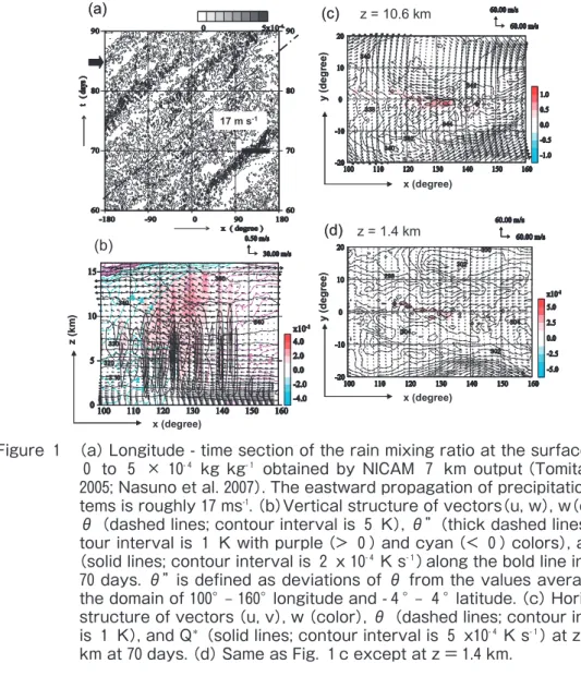
of the NICAM aqua-planet simulation are utilized. Two outputs are usable: 3-hourly averaged data with a zontal grid size of 7 km and snapshot data with a hori-zontal grid size of 3.5 km at 85 days(marked by an arrow in Fig. 1a). Figure 1a shows a longitude-time sec-tion of the rain mixing ratio at the surface in the NICAM 7 km outputs(Tomita et al. 2005; Nasuno et al. 2007). EP disturbances similar to the observed SCs with a speed of 17 ms-1, as well as WP cloud clusters, are well reproduced. These features are discussed in detail in Nasuno et al.(2007, 2008). A vertical section of u, w, θ , θ”, and Q* at 70 days along the line of 100° –160° longitude is shown in Fig. 1b. θ” is defined as the deviations of θ from the values averaged in the horizontal domain(100° – 160° longitude and -4° – 4° latitude in this case). Variables averaged in 1 degree are used to demonstrate the general features of SCs.
(9) ∆θ exp { −(x / xa )2 −(y / ya )2 } cos {π (z −za) / (2za ) }, (d) z = 1.4 km (c) z = 10.6 km x (degree) x (degree) y (d eg ree ) y (d eg ree ) 17 m s-1 (a) (b) x (degree) z (k m ) 1 (d) z = 1.4 km (c) z = 10.6 km x (degree) x (degree) y (d eg ree ) y (d eg ree ) 17 m s-1 (a) (b) x (degree) z (k m ) 1
Figure 1 (a)Longitude - time section of the rain mixing ratio at the surface from 0 to 5 × 10- 4 kg kg- 1 obtained by NICAM 7 km output(Tomita et al 2005; Nasuno et al. 2007). The eastward propagation of precipitation sys-tems is roughly 17 ms-1. (b)Vertical structure of vectors(u, w), w(color), θ(dashed lines; contour interval is 5 K), θ”(thick dashed lines; con-tour interval is 1 K with purple(> 0 )and cyan(< 0 )colors), and Q* (solid lines; contour interval is 2 x 10- 4 K s- 1)along the bold line in(a)at
70 days. θ” is defined as deviations of θ from the values averaged in the domain of 100° – 160° longitude and - 4 ° – 4 ° latitude. (c)Horizontal structure of vectors(u, v), w(color), θ(dashed lines; contour interval is 1 K), and Q*(solid lines; contour interval is 5 x10- 4 K s- 1)at z = 10.6 km at 70 days. (d)Same as Fig. 1 c except at z = 1.4 km.
The main diabatic heating occurs at an interval of 115° – 145° longitude, and SCs are seen in this range. Warm (cold)θ” is located on the eastern(western)side of
the heating. Figures 1c and 1d show the horizontal pat-terns of u, v, w, θ , and Q* at the heights of 10.6 km and 1.4 km, respectively. Convergence at z = 1.4 km and divergence at 10.6 km are found around the areas of upward motions. It is noteworthy that the off-equato-rial vortices found on both sides of upward motions, which are an equatorial Rossby wave-like response pat-tern, are seen, especially remarkably on the northern hemisphere at z = 10.6 km. These features can be obtained at any time; however, they are more remark-able when the diabatic heating is localized like around 70 days. In this way, the large-scale horizontal struc-tures obtained by the NICAM generally look like a Gill (1980)response pattern.
The domains(Lx, Ly)are specified for the calculation of the basic fields. Figure 2 shows the vertical profiles
of <Q*>, <w>, < θ >, < u >, and <ρ>. The vertical profiles denoted by solid lines are selected by averaging the domain of 40°– 50° longitude(Lx = 10°)and -4°– 4° latitude(Ly = 8°)from snapshot data of 3.5 km at 85 days. In this area, the most intensive precipitation is related to the EP disturbance. Compared with those in the 7-km resolution in the same domain at 85 days, Q* and w are stronger in intensity by more than 2. How-ever, similar shape and intensity for Q* are obtained at 70 days, when the isolated heating is remarkable. 3. Results of a full model and its comparison
with NICAM outputs
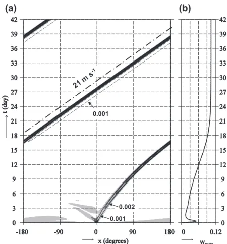
Hereafter, the outputs of a full model are presented. Figure 3a is a longitude - time section of W’ along the equator at z = 3.7 km. At the initial time, simulated dis-turbances split in both eastward and westward direc-tions, but the WP disturbance soon disappears, while
(a) (d) (c) (b) <Q*> <w> <ρ> <θ> <u> <θ> <θ> <ρ> <θ>
Figure 2 Mean vertical profiles of(a)Q* ,(b)w ,(c)θ , and(d)u and ρ. Solid lines denote variables averaged in the domain of 40°– 50° longitude and - 4 °– 4 °latitude at 85 days obtained by NICAM 3.5 km output. Dotted lines in(a)and(b)mean variables averaged in the same domain and days as the solid lines, except NICAM 7 km output. Dashed lines in(a),(b)and (d)denote variables averaged in the domain of 115 °– 145 ° longitude and
the EP one becomes dominant as a single disturbance. It is noteworthy that the EP speed is slow at first (about 9.6 ms-1), then becomes fast, and is finally uni-form(about 21 ms-1)after about 15 days. The round-the-world time is approximately 21 days by using this speed. Figure 3b is a temporal variation of the maxi-mum values of W’ at z = 3.7 km. Maximaxi-mum values grow with time and become saturated and then uniform after about 20 days. The final propagation speed of a pre-ferred disturbance is synchronously related to its maxi-mum amplitude.
It is noteworthy that the horizontal structure, con-sisting of a single small area of intense upward motion and widespread areas of weak downward ones, is established after about 4 days. Such a feature is fre-quently found in the POWC-type cases(e.g., Lau and Peng 1987)and is also similar to the stage around 70 days in Fig. 1a, in which one intense precipitation area
is dominant.
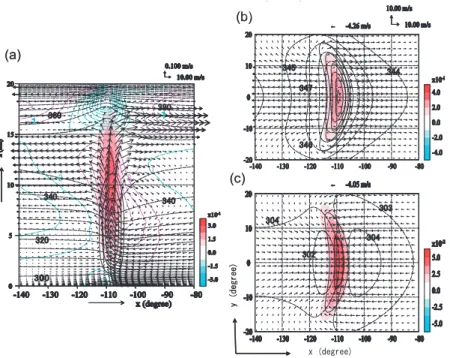
The vertical section of U, W’, θ , θ”, and Q* is shown in Fig. 4a. The upright feature of convection reaching a height of 17 – 18 km is seen, and conver-gence(divergence)in the lower(upper)troposphere is found. Different heights of the intense updraft are noticed on the eastern and western sides(about 18 km and about 15 km, respectively). Slightly leftward tilting of θ” is also found with a height below 15 km. The horizontal sections of U’, V’, W’, θ , and Q* at the heights of 10.4 km and 1.4 km are shown in Figs. 4b and 4c, respectively. A baroclinic structure is obvious. The Kelvin wave-like response pattern is noticed on the eastern side of the heating, while the equatorial Rossby wave-like off-equatorial gyres are remarkable on the western side. These features are similar to the Gill (1980)response pattern, as anticipated from the PS
view.
(a)
(b)
wmax 0.001 0.002 0.001Figure 3 (a)Longitude - time section of W at the equator at z = 3.7 km in the full model with the same grid location as the NICAM and the basic fields obtained by the NICAM aqua-planet simulation. Areas of upward and downward motions are drawn by solid and dashed lines with contour interval of 10- 3 ms-1, respectively. Areas drawn by grey indicate those of upward motion.(b)Temporal variation of the maximum W at z = 3.7 km.
Here, the propagation speed and structures are com-pared with those of the NICAM aqua-planet simulation. The propagation speed in this case is 21 ms-1 and is con-sidered to be a similar magnitude to that in Fig. 1a (Tomita et al. 2005; Nasuno et al. 2007), because both
are in the range of 15 – 25 ms-1 of observed SCs in Wheeler and Kiladis(1999). For the vertical structure, the upright features of upward motions and θ” are remarkable in Fig. 4a compared with Fig. 1b and the results of Nasuno et al.(2008). These are due to a com-pact distribution of the diabatic heating in the longitudi-nal direction.
For the horizontal structure, a similar pattern about the wind fields, especially in the upper troposphere (Fig. 4b), is found to that of Fig. 1c: the dominant Kel-vin wave-like zonal wind on the eastern side of the heating and the equatorial Rossby wave-like off-equato-rial vortical circulation on the western side. However, a large latitudinal extension of Q* and W’ is noticed in Figs. 4b and 4c, while time-dependent scattered meso-scale(~100 km)heating is seen aligned along the
equa-tor in Figs. 1c and 1d. This difference may come from whether the Hadley circulation exist(Fig. 3)or not (Figs. 4 and 5). In spite of this difference, the wind
fields are similar to large-scale response patterns as reported above. The question of why similar wind fields are induced by different extensions of the heating needs to be asked. Linear steady response problems of large-scale and mesolarge-scale heating are studied in Appendix. From this study, large-scale response patterns of winds are obtained similarly even when the mesoscale heating is specified to be aligned in the longitudinal or latitudi-nal direction. Therefore, it is concluded that the differ-ence of horizontal extension of the heating is not serious as far as detailed differences are not concerned. A full model reproduces the EP property and asym-metric east-west structure. However, it does not simu-late observed features, such as a MSS and vertically slanted structures of PSs(e.g., Nakazawa 1988). These may stem from the large horizontal diffusion / viscosity and a simultaneous adjustment time of the POWC adopted in this study. Due to large horizontal diffusion /
x (degree) y ( d e g ree ) (c) 0 -2 -1 -1 1 2 3 (b) 1 2 (b) (c) (a) x (degree) y ( d e g ree ) (c) 0 (c) -2 -1 -1 1 2 3 (b) 1 2 (b) 1 2 (b) (c) (a)
Figure 4 (a)Vertical structure of vectors(U, W’), W’(color), θ(dashed lines; contour interval is 5 K), θ”(thick dashed lines; contour interval is 1 K with purple(> 0 )and cyan(< 0 )colors), and Q*(solid lines; contour interval is 10- 4 K s- 1)along the equator at 21 days. θ” is defined as deviations of θ from the values averaged in the domain of -140° – -80 °longitude and - 4 ° – 4 ° latitude.(b)Horizontal struc-ture of vectors(U, V’), W’(color), θ(dashed lines; contour interval is 1 K), and Q*(solid lines; contour interval is 10- 4 K s- 1)at z = 10.6 km at 21 days.(c)Same as Fig. 1 c except at z = 1.4 km.
viscosity, the large-scale preferred disturbance is uniquely selected, resulting in neither smaller-scale ones nor a MSS. In addition, the simultaneous adjustment time of the POWC might produce vertically upright structures.
4. Simplification by changing the model and basic fields
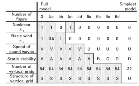
The full model used in Section 3 had the same struc-ture and number of vertical grid points as those of NICAM, and the basic fields of u, θ, and ρ obtained by the NICAM are also used. Owing to these treatments, the EP property was obtained. However, the full model still has various factors, such as the nonlinear terms, basic zonal wind and so on. To that end, the full model is simplified step-by-step, eliminating the nonlinear terms and basic zonal wind and modifying the basic fields of a speed of sound waves and static stability. <N> is the horizontally averaged static stability defined as . The simplification process is shown in Table 1.
a. Elimination of the nonlinear terms and basic zonal wind
Here, simplification starts by changing the values of ε1 and ε2. The W-field and the maximum values in the nonlinear cases with half the basic zonal wind and with-out it are shown in Figs. 5a and 5c, respectively. Com-pared with Fig. 3a, the basic zonal wind still works for the development of the EP disturbance. In a linear case, a preferred disturbance with a maximum growth rate increases exponentially with time, and, thus, logarithmic forms of w are utilized for plotting. The log 10 |w| fields in the linear cases with and without the basic zonal wind are shown in Figs. 5b and 5d, respectively. Even in these cases, the basic zonal wind plays a supporting role on the EP property. It is concluded that both the nonlinear terms and basic zonal wind play a consider-able role on the maintenance of EP property.
b. Modification of the basic fields of a speed of sound waves and static stability
The basic fields of the speed of sound waves and static stability are further modified. In Fig. 6a, the basic field of <Cs>, where the original one varies with an amplitude of about 40 ms-1 around 300 ms-1 in the tropo-sphere(not shown), changes into a uniform one(300
z g N = ∂∂θ
θ
Table 1 Simplification processes. The model becomes simpler from left to right. The parameters of ε1 and ε2 are specified 1 or 0.5 or 0. The symbols of V, U, and S denotes “variable”, “uniform”, and “stretched”, respectively. A, B, C, and D of static stability means Lines A, B, C, and D in Fig.7, respectively. The boundaries from grey areas to white ones denote changes of model or basic fields.
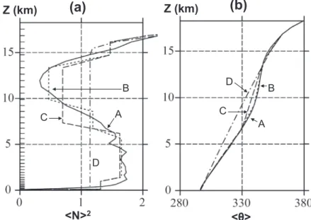
ms-1). In this case, its impact is small. On the other hand, the change of <N>2 has a large impact on the EP property. Figures 7a and 7b show the vertical profiles of <N>2 and θ , respectively. Line A in Fig. 7 refers to the original <N>2 case, and a wavy structure between 0 and 16 km(called “troposphere”)are obvious: <N>2 has large values in the lower layer(called “lower tropo-sphere”)and small values in the upper layer(called “upper troposphere”). Line B is the approximation of the original <N>2, and Line C is a smaller amplitude of
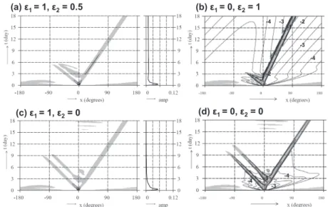
the wavy structure than that of Line B. Line D is a uni-form <N>2 case. Figures 6b, 6c, and 6d correspond to the cases of Lines B, C, and D, respectively. In Figs. 6b and 6c, the EP property remains, although it weakens. However, a single WP disturbance appears in Fig. 6d when the uniform <N>2 is specified. It is noteworthy that the growing disturbance appears only in Fig. 6d, while all EP and WP disturbances are seen in Figs. 5 and 6a, 6b, and 6c, although they decay with time. Therefore, a different propagation regime appears
(a) ε1 = 1, ε2= 0.5 (c) ε1 = 1, ε2= 0 (d) ε1 = 0, ε2= 0 -3 -4 -3 -4 (b) ε1 = 0, ε2= 1 -3 -2 -3 -4 -4 -2 -1
Figure 5 (a)Longitude - time section of W and the maximum values at the equator at z = 3.7 km for the nonlinear case with a half of basic wind.(c)Same as(a)except no basic wind.(b)Longitude - time section of log 10 | w | at the equator at z = 3.7 km for the linear case with the basic wind.(d)Same as(b)except no basic wind. Areas drawn by grey indicate those of upward motion.
-3 -4 -4 -3 (a) (b) (c) (d) -4 -2 -4 -3 -3 -3 -3 -4 -4 -3 -4 -3 8 2 6 4 10 14 16
Figure 6 (a)Longitude - time section of log 10 | w | at the equator at z = 3.7 km with a uniform Cs for(a)original <N>2 case(Line A in Fig. 7 ),(b) approximated <N>2 one(Line B in Fig. 7 ),(c)smaller <N>2 one (Line C in Fig. 7 ), and(d)uniform <N>2 one(Line D in Fig. 7 ),
when the wavy structure of <N>2 disappears. The rea-son for the disappearance of the EP property in the uni-form <N>2 case will be discussed in the next subsection.
c. Reason for the disappearance of the EP prop-erty in a uniform <N>2 case
Modifying(4), the buoyancy equation can be derived. Here, only the fi rst term of the right hand side are written as
From Fig. 7(Line A), <N>2 in the troposphere can be approximated as the sum of a constant part <N>02 and variable part <N>12 as
<N>12 is simply assumed to be a sinusoidal function of z, where α is a positive constant and zM is roughly 8 km (Fig. 8). The vertical velocity is roughly represented
as
where W0 is a positive constant and G(x, y)means the horizontal function. Then, the buoyancy equation(10) can be rewritten, excluding the horizontal part, as
Here, only the second term on right-hand side is dis-cussed. It is noteworthy that –W’<N>12 has positive val-ues in the upper troposphere and negative ones in the lower one. This term works as the heating(cooling)in the upper(lower)troposphere in the buoyancy equation. That is, the vertical advection of <N>12 has the same
(10) ... 2+ ′ − = ∂ ′ ∂ W N t B (11)
(
)
. sin , 2 1 2 1 2 0 2 − − ≈ + ≡ M M z z z N where N N N α π (12)(
)
( , ) 2 cos ' W0 zz z G x y W M M − ≈ π (13)(
)
(
)
... 2 sin 2 3 sin 2 0 + − + − + M M M M z z z z z z Wα π π(
)
2 cos ... 2 0 0 2 1 2 0 − − ⇒ + ′ − ′ − = ∂ ′ ∂ M M N z z z W N W N W t B π(b)
A B D C(a)
A B C DZ (km)
Z (km)
<N>
2<θ>
Figure 7 Vertical profi les of(a)<N>2(unit: 10- 4 s- 2)and(b)< θ >(unit: K). Lines A, B, C, and D denote original, approximated, smaller <N>12, and uniform cases, respectively. <N>12 means a devia-tion of static stability from the constant value.
Figure 8 Schematic profi les of W’, <N>12, and –W’<N>12.
role as the top-heavy heating case. The conclusion obtained here, in which the reduction of <N>2 variation is connected to the weakening of the EP property, is consistent with the result that splitting disturbances likely occur in the top-heavy heating, which will be dis-cussed in Part 2.
5. Discussion and summary
The EP property of SCs in the equatorial areas is interesting and important problems. Thorough explana-tions will lead to an understanding of the fundamental physics of tropical meteorology. To explain the EP property of SCs as simply as possible, the POWC was adopted.
A full model, which has the same structure and num-ber of vertical grid points as those of the NICAM as well as basic fields obtained by the NICAM outputs, was first applied. A finite-amplitude EP disturbance is attained with a speed of about 21 ms-1, comparable to the NICAM outputs. Its horizontal structure indicates the asymmetric structure in the longitudinal direction, similarly to the Gill response pattern, i.e., the Kelvin wave-like zonal patterns on the eastern side of the dis-turbance and the equatorial Rossby wave-like off-equa-torial vortical patterns on the western side. When Figs. 1c/1d and 4b/4c are compared, however, a large differ-ence in the horizontal distributions of the heating is noticed, i.e., the mesoscale heating aligned along the equator obtained by the NICAM and the large-scale heating obtained by the full model. The linear responses of winds for the various horizontal exten-sions of the heating are compared. It is shown that sim-ilar horizontal patterns of winds are obtained in spite of the various extensions of the heating and, thus, this dif-ference does not seriously affect the conclusion.
Next, simplification of the full model is pursued to achieve a deep understanding of the EP property. The following steps are conducted; eliminating the nonlinear terms and basic zonal wind and modifying the basic fields of a speed of sound waves and static stability. It is shown that the EP disturbance changes into a WP one when the static stability becomes uniform, which origi-nally has a wavy structure in the troposphere with
large(small)values in the lower(upper)troposphere. The vertical advection of variable static stability has the same role to enhance the top-heavy heating.
In Part 2, using a simplest model, which is a different standpoint from this study, two propagation regimes and their formation mechanism is discussed. In the sim-plest model, a slowly WP disturbance is anticipated in the ‘usual’ observed heating profiles, differently from the preferential EP disturbances in the full model. The connection of the results in Parts 1 and 2 is one of the concerns.
Acknowledgements
The author is deeply indebted to Drs. T. Nasuno, Japan Agency for Marine-Earth Science and Technolo gy (JAMSTEC)and H. Tomita, RIKEN, and Prof. M. Satoh, University of Tokyo / JAMSTEC, for the use of the NICAM outputs and many discussions. Thanks are extended to Drs. T. Nozawa, Okayama University and T. Horinouchi, Hokkaido University for giving many comments for improving the manuscript.
Appendix
A linear response problem about the localized steady heating is studied assuming an equatorial beta plane and hydrostatic approximation. The forcing Q is pre-scribed as functional forms. Considering a vertical mode and assuming an infinite <Cs>, constant < θ > except for static stability, and constant <ρ> in(1) - (5), non-dimensional governing equations are given as
Here, non-dimensional variables are denoted by asteri-sks. Non-dimensional units of horizontal distance(NH/2 βπ)1/2 and time(π/2β NH)1/2 roughly correspond to
1,050 km and 5.7 hr in dimensional forms, respectively,
(A1) , 2 1 * * * * * * * * u x p v y t u − ∂ ∂ − = ∂ ∂ λ (A2) , 2 1 * * * * * * * * v y p u y t v − ∂ ∂ − − = ∂ ∂ λ (A3) , * * * * * * * * * Q p y v x u t p − − ∂ ∂ − ∂ ∂ − = ∂ ∂ λ (A4) . * * * * p Q w =λ +
when N = 10-2 s-2, H = 16 km, and β = 2.3x10⁻¹¹ m-1 s-1 are used. Gill(1980, 1982)obtained large-scale response pat-terns assuming a long-wave approximation, where the left-hand side of(A2)is neglected. In this case, a time-integration is adopted as an initial value problem with-out such assumption. A symmetric heating profile abwith-out the equator(y* = 0)in the latitudinal direction is speci-fied. The closed domain is used between the range of (-25, 25)in the longitudinal direction and(0, 5)in the
latitudinal one. The grid sizes Δ x* and Δ y* are 0.01, and the time step Δ t* is 0.01. The time-integration is performed until t* = 10, when the reflection of gravity waves from the boundaries does not significantly affect
this simulation.
Figure A1 shows snapshops of horizontal winds and p*, which corresponds to -θ’ in the lower troposphere, at the lower layer at t* = 2 and t* = 7. The mesoscale heating with a square size of 0.1 is specified as(a)a piece on the equator,(b)three pieces aligned along the equator with an interval of 0.4, and(c)three pieces aligned along the latitude with an interval of 0.4. On the other hand, the large-scale heating with a Gaussian shape is specified in(d). At t* = 2, the initial impulse is seen, especially in(a), around the radius of 2 from the (0, 0)point. The inner areas correspond to influence
regions. Hereafter, our focus is limited to t* = 7, when
(a) t
*= 2
t
*= 7
(b) t
*= 2
t
*= 7
(c) t
*= 2
t
*= 7
(d) t
*= 2
t
*= 7
Figure A 1 Horizontal distributions of horizontal winds and p*’ at the lower layer at t* = 2 and t* = 7 for(a)one-piece mesoscale heating case with a square size of 0.1 on the equator,(b)three-piece mesoscale heating case with an interval of 0.4 along the equator,(c)three-equator,(b)three-piece mesoscale heating case with an interval of 0.4 along the latitude, and(d)large-scale heat-ing case with a Gaussian shape. In(d), the forcheat-ing is denoted by solid lines with an interval of 0.2. The heating is assumed to be symmetric about the equator(y* = 0 )and drawn by bold solid lines. The dashed lines of negative p*’ are drawn with an interval of 0.2. The scales in each figure are normalized arbitrary. Winds are plotted with an interval of 0.1.
nearly steady fields are attained. When four figures are compared, the details, such as vortical motions near the heating, are different. However, when large-scale fea-tures are compared, it is indicated that the Kelvin wave-like zonal winds are dominant on the eastern side of the heating, while an equatorial Rossby wave-like vortical circulation off the equator is predominant on the western side. In other words, asymmetric horizon-tal structures due to the equatorial beta are seen even when the size of the heating is small. It is concluded that the difference of the heating extension is not seri-ous.
References
Bretherton, C. S., 2002: Wave-CISK. In Vol. 3 of Encyclopedia of Atmospheric Sciences, edited by J. R. Holton, J. A. Curry and J. A. Pyle, Academic Press, 1019-1022.
Gill, A. E., 1980: Some simple solutions for heat-induced trop-ical circulation. Quart. J. Roy. Meteor. Soc., 106, 447-462. Gill, A. E., 1982: Atmosphere-Ocean Dynamics. Academic
Press, 662pp.
Hayashi, Y, -Y. and A. Sumi, 1986: The 30-40 day oscillations simulated in an “aqua-planet” model. J. Meteor. Soc. Japan, 64, 451-467.
Lau, K. –M. and L. Peng, 1987: Origin of low-frequency (intraseasonal)oscillations in the tropical atmosphere.
Part I: Basic theory. J. Atmos. Sci., 44, 950-972.
Louis, J., 1979: A parameteric model of vertical eddy fluxes in the atmosphere. Boundary Layer Meteor., 17, 187-202. Khouider, B. and A. J. Majda, 2006: A simple multicloud
parameterization for convectively coupled tropical waves. Part 1: Linear analysis. J. Atmos. Sci., 63, 1308-1323. Madden, R. and P. Julian, 1971: Detection of a 40-50 day
oscillation in the zonal wind in the tropical Pacific. J. Atmos. Sci., 28, 702-708.
Majda, A. J. and M. G. Shefter, 2001: Waves and instabilities for model tropical convective parameterizations. J. Atmos. Sci., 58, 896-914.
Majda, A. J., B. Khouider, G. N. Kiladis, K. H. Strayb and M. G. Shefter, 2004: A model for convectively coupled tropical waves: Nonlinearity, rotation, an comparison with obser-vations. J. Atmos. Sci., 61, 2188-2205.
Mapes, B. E., 2000: Convective inhibition, subgrid-scale trig-gering energy, and stratiform instability in a toy tropical wave model. J. Atmos. Sci., 57, 1515-1535.
Mellor, G. L. and T. Yamada, 1974: A hierarchy of turbu-lence closure models for planetary boundary layers. J. Atmos. Sci., 61, 1521-1538.
Nakajima, K. and T. Matsuno, 1988: Numerical experiments concerning the origin of cloud clusters in the tropical atmosphere. J. Meteor. Soc. Japan, 66, 309-329.
Nakajima, T., M. Tsukamoto, Y. Tsushima, A. Numaguti, and T. Kimura, 2000: Modeling of the radiative process in an atmospheric general circulation model. Appl. Opt., 39, 4869-4878.
Nakazawa, T., 1988: Tropical super clusters within intrasea-sonal variations over the western Pacific. J. Meteor. Soc. Japan, 66, 823-839.
Nasuno, T., H. Tomita, S. Iga, H. Miura and M. Satoh, 2007: Multiscale organization of convection simulated with explicit cloud processes on an aquaplanet. J. Atmos. Sci., 64, 1902-1921.
Nasuno, T., H. Tomita, S. Iga, H. Miura and M. Satoh, 2008: Convectively coupled equatorial waves simulated on an aquaplanet in a global nonhydrostatic experiment. J. Atmos. Sci., 65, 1246 -1265.
Neelin, J. D., I. M. Held and K. H. Cook, 1987: Evaporation-wind feedback and low-frequency variability in the tropi-cal atmosphere. J. Atmos. Sci., 44, 2341-2348.
Raymond, D. J., S. L. Sessians, A. H. Sobel and Z. Fuchs, 2009; The mechanics of gross moist stability. J. Adv. Model. Earth Syst., 1, 1-20.
Saito, K., T. Fujita, Y. Yamada, J. Ishida, Y. Kumagai, K. Aranami, S. Ohmori, R. Nagasawa, S. Kumaga, C. Muroi, T. Kato, H. Eito and Y. Yamazaki, 2006: The operational JMA nonhydrostatic mesoscale model. Mon. Wea. Rev., 134, 1266-1298.
Satoh, M., 2003: Conservative scheme for a compressible nonhydrostatic model with moist processes. Mon. Wea. Rev., 131, 1033-1050.
Smith, R. N. B., 1990: A scheme for predicting layer clouds and their water content in a general circulation model. Quart. J. Roy. Meteor. Soc., 116, 435-460.
Takahashi, M., 1987: A theory of the slow phase speed of the intraseasonal oscillation using the wave-CISK. J. Meteor. Soc. Japan, 65, 43-49.
Takayabu, N. Y., 1994: Large-scale cloud disturbances associ-ated with equatorial waves. Part I: Spectral features of the cloud disturbances. J. Meteor. Soc. Japan, 72, 433-449. Tomita, H., H. Miura, S. Iga, T. Nasuno and M. Satoh, 2005:
A global cloud-resolving simulation: Preliminary results from an aqua planet experiment. Geophy. Res. Lett., 32, L08805, doi: 10.1029/2005GL022459
Wang, B. and T. Li, 1994: Convective interaction with bounda-ry-layer dynamics in the development of a tropical intra-seasonal system. J. Atmos. Sci., 51, 1386-1400.
Wang, B., 2005: Theory, in Intraseasonal Variability in the Atmosphere-Ocean Climate System, edited by W. K. M.
Lau and D. E. Waliser, pp307-360, Praxis, Chichester, U.K. Wheeler, M. and G. N. Kiladis, 1999: Convectively coupled
equatorial waves: Analysis of clouds and temperature in the wavenumber-frequency domain. J. Atmos. Sci., 56, 374-399.
Yang, G. -Y., B. Hoskins and J. Slingo, 2007: Convectively coupled equatorial waves. Part. II: Propagation character-istics. J. Atmos. Sci., 64, 3424-3437
Yano, J. -I, J. C. McWilliams. M. W. Moncrieff and K. A. Emanuel, 1995: Hierarchical tropical cloud systems in an analog shallow-water model. J. Atmos. Sci., 52, 1723-1742. Yoshizaki, M. and A. Mori, 1990: Another approach on linear
theory of conditionally unstable convection. J. Meteor. Soc. Japan, 68, 327-334.
Yoshizaki, M., 1991a: Selective amplification of the eastward- propagating mode in a positive-only wave-CISK model on an equatorial beta plane. J. Meteor. Soc. Japan, 69, 353-373. Yoshizaki, M., 1991b: On the selection of eastward-propagat-ing modes appeareastward-propagat-ing in the wave-CISK model as tropical intraseasonal(30-60-day)oscillations. -Linear response to localized heating moving in the east-west direction on an equatorial beta plane. J. Meteor. Soc. Japan, 69, 595-608. Yoshizaki, M., S. Iga and, M. Satoh, 2012a:
Eastward-propa-gating property of large-scale precipitation systems
simu-lated in the coarse-resolution NICAM and an explanation of its appearance. SOLA, 8, 21-24.
Yoshizaki, M., K. Yasunaga, S. Iga, M. Satoh, T. Nasuno, A. T. Noda, and H. Tomita, 2012b: Why do super clusters and Madden Julian Oscillation exist over the equatorial regions? SOLA, 8, 33-36.
Yoshizaki, M., 2016: Comparison of models having positive-only wave CISK with the NICAM outputs about eastward propagation of super clusters in the equatorial region: Part 2. Approach from a simplest model. Bulletin of Geo-Environmental Sci., 18, 17-27.
Footnotes:
1)‘Negative precipitation’ is hard to imagine because real precipitation is irreversible. Therefore, PSs with ‘nega-tive precipitation’ should be considered to be fictitious ones.
2)The values of static stability and speed of sound waves are independently treated, although they should be inter-related.
3)In this study, the term “nonlinearity” is used when(7) and(8)are included, although the POWC itself has nonlin-earity in the horizontal direction.
赤道域のスーパークラスタの東進に関する NICAM の計算結果と positive-only
wave CISK を持つモデルの比較. Part 1. フルモデルからのアプローチ
吉 𥔎 正 憲*
*立正大学 ・ 地球環境科学部
要 旨:
赤道対称モードの大規模東進じょう乱として、1000km オーダーの水平スケールをもち15 – 25 ms-1の速度のスーパー
クラスタ(SC)と5000km オーダーの水平スケールを持ち10 ms-1以下の速度のマッデンジュリアン振動が観測される
(Wheeler and Kiladis 1999)。positive-only wave CISK を使うと、top-heavy な熱源分布のとき、東西に分裂するじょ う乱が発生しいずれ東進じょう乱が卓越する(Yoshizaki, 1991a, Yoshizaki et al 2012b)。しかし、単純なモデルで単 純な環境場を与えると、伝搬性のじょう乱は‘非常に大きな’top-heavy な熱源分布の場合にしか発現しない。ここ では、‘もっともらしい大きさ’の top-heavy な熱源分布で伝搬性のじょう乱が得られることを目指した。 NICAM と同じ鉛直グリッドと環境場を持つフルモデルを用いることによって、Gill(1980)パターンと同じような 東西に非対称な構造の東進擾乱を再現し、また NICAM 出力と同じような東進速度をもつことを示した。さらに非線 型項や基本場の東西風を消去したり音波や大気安定度の大きさを変えたりする実験を行い、東進する擾乱がゆっくり と西進するものに急変するのは、対流圏下層では大きく対流圏上層では小さい大気安定度を鉛直一様にするときに起 こることがわかった。その理由は、大気安定度の鉛直方向の依存性が top-heavy な熱源分布を強化するためである。 これから、単純な環境場から大気安定度を実況に近いものに変えることにより、 ‘通常’の top-heavy な熱源分布でも 伝搬性のじょう乱が得られると期待される。