Analysis on the Distribution of COVID-19 Cases by Country

Analysis on the Distribution of COVID‑19 Cases by Country

雑誌名 福井大学学術研究院工学系部門研究報告

巻 69

ページ 37‑41

発行年 2021‑03‑26

URL http://hdl.handle.net/10098/00028627

Analysis on the Distribution of COVID-19 Cases by Country

(Received December 21, 2020)

The global cases of COVID-19 reported on the website of Center for Systems Science and Engineering at Johns Hopkins University are used to analyze the distribution by country. The relationship between rank and size (ranking plot) is approximately represented by the power-law distribution for the top countries, while the overall distribution follows the lognormal distribution.

Assuming a continuous power-law distribution, the power exponent determined from the data leads to make the weight average infinity, which would be considered as gelation or pandemic. The distribution is rationalized by the discrete-time stochastic model that employs the weekly reproduction rate µ. The distribution of µ obtained for the time period, between April 20 and November 11, 2020 could be approximated by the gamma distribution. By assuming a gamma distribution for µ with various pairs of average and variance, the required conditions to stop the pandemic are (1) the average µ must be smaller than unity and (2) the time period for µ > 2 must be negligibly small.

Key Words : COVID-19, Ranking Plot, Power Law, Lognormal Distribution, Pandemic, Weekly Reproduction Rate

1. Introduction

On April 7, 2020, the Japanese government declared a state of emergency for the rapid spread of COVID-19 in Japan. On that weekend, one of the authors (HT) was staring abstractedly at the website of Center for Systems Science and Engineering at Johns Hopkins University,^[1]

listing a large number of the COVID-19 cases by country.

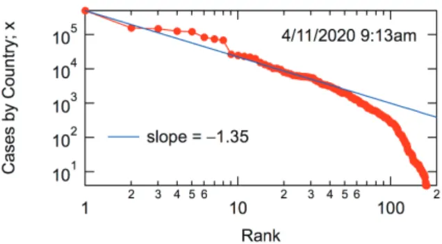
Simply because there are so many numbers, HT examined the numbers, and tried the ranking plot, graphically showing the relationship between rank and size. Figure 1 shows the double logarithmic plot made at that time. Interestingly, the top countries appear to follow the power-law relationship. Recalling his own experience that a power law was found also in the infection tree of SARS in 2003,^[2] and intrigued by the Zipf’s law like behavior, HT called for a volunteer to collect the data, and an undergraduate student, MF applied for this project.

* Department of Materials Science and Engineering

**Department of Materials Science and Biotechnology, School of Engineering

Fig. 1 Conventional ranking plot.

Fig. 1 shows a conventional type of ranking plot in which the y-axis shows the size and the x-axis shows the rank. Because the rank is proportional to the number fraction of countries whose size is larger than the corresponding size, when the axes are exchanged to plot the rank on the y-axis, the ranking plot shows the upper probability distribution given as follows.

Rank∝ N(x)dx

x

∫

In Eq. (1), N(x) shows the number-based probability density function (pdf). In the rest of this article, the rank is shown on the y-axis, representing the upper probability distribution.

Mem. Fac. Eng. Univ. Fukui, Vol. 69（March 2021）

The collected data from the website^[1] during the period from April 11 to November 11, 2020 are analyzed.

A discrete-time stochastic model proposed by Yamamoto^[3] is used to rationalize the formation process of the obtained distribution. Based on the analysis, the necessary conditions to stop the pandemic are proposed.

2. Analysis of Distribution Data

2.1 Power-Law Distribution

Fig. 2 shows the ranking plot on the designated date.

The power law seems to apply for the top countries, irrespective of the dates.

N(x)dx

x

∫

Fig. 2 Ranking plots on the designated dates.

The power exponent, α is approximately in the range of 0.7 – 0.9. Based on Eq. (2), the upper tail of the number-based pdf, N(x) is represented by:

N(x)∼x^{−α −1} for large x’s. (3)

An interesting characteristic of the power-law distribution is that when the pdf is converted to that on a weight basis W(x), the power exponent changes by one.

W(x)∼x^−α for large x’s. (4) Equation (4) shows that the power exponent of the ranking plot is directly equal to the power exponent of the weight-based pdf.

Assuming a continuous distribution, the weight average is obtained from the following equation.

x_w =

∫

∫

Equation (5) shows that when the exponent (–α +1) is greater than or equal to –1, the integration goes to infinity. Therefore, the critical value of α is 2.

The weight average is the expected size of the cluster when a unit is selected randomly, which corresponds to

the onset of gelation in the polymer science.^[4] In order for the expected cluster size to stay finite, α must be larger than 2. On the other hand, however, the obtained α-values are always smaller than 2 during the whole investigated period. This could be interpreted as pandemic.

2.2 Lognormal Distribution

Although the upper tail probability distribution could be represented by the power law reasonably well, the whole distribution, including the lower-ranked countries, is not.

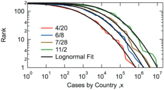
Fig. 3 shows the least-square fit by using the lognormal distribution. The whole distribution is well represented by the lognormal distribution.

Fig. 3 Fitted curves by using the lognormal distribution.

Recently, it has been argued that many power-law distributions reported earlier both for the social and natural sciences are just apparent, and do not fully conform to a strict power law,^[5] and many of them are better represented by the lognormal distribution.^[6] It is not straightforward to distinguish these two types of distribution. In this article, we do not go into the details of statistical discrimination. We just report the following two notable characteristics of the ranking plot of COVID-19: (1) the top countries appear to follow the power-law distribution, and (2) the overall distribution could be represented by the lognormal distribution.

3. Model-Based Investigation to Elucidate the Ranking Plot

In COVID-19, the patients are isolated once they are found to be positive. Therefore, the infectious period is limited. Although there may be many hidden patients that are not counted as the cases reported on the Johns Hopkins’ website, we consider only the numbers reported therein.

38

We employ a discrete-time stochastic model. Suppose the increase of cases during a certain period of time is Δxt, and the increase in the next time period is Δxt+1. The newly infected would be infectious, and let µt be the apparent reproduction rate, defined by:

µ_t = Δx_t+1 Δx_t. (6) With the present simple model, the number of cases xt

is represented by the following equations.

x^t+1=x_t+ Δx_t. (7)

Δx_t=µ_t−1Δx_t−1. (8) Yamamoto^[3] investigated the present model, and found that x has a stationary power-law tail with x^−α, if the following equation possesses a unique positive solution.

E(µ_t^α)=1. (9)

where E represents the expectation of the distribution.

Therefore, Eq. (9) is equivalent to:

µ^α f(µ)dµ

0

∫

where f is the pdf of µ.

The reported COVID-19 data showed a weekly fluctuation: the number tends to be small every Monday.

In addition, one week would be a reasonable infectious time period, and we employ the weekly reproduction rate.

Fig. 4 Distribution of the weekly reproduction rate µ.

The histogram shown in Fig. 4 is the pdf of the weekly reproduction rate µ observed during the period, from April 20 to November 11, 2020. The data for the top 120 countries on October 17 are used. Note that the data of the lower ranked countries tend to involve Δxt = 0, as well as µ with extraordinary large magnitude. In addition,

because the frequency to have µ > 4 is so small, we neglected such data to determine the µ distribution. The solid line shows the interpolation curve, connecting the center points of the histogram. This curve is used for the Monte Carlo (MC) simulation.

In the MC simulation, the total number of countries is set to be N = 190, which is equal to that of the obtained data for the most of the investigated period. The initial values are set to be x0 = 0 and Δx-1 = 1 for all countries.

Fig. 5 shows the MC simulation results after 50 weeks.

Even though the initial values are the same for all countries, a wide variation among countries is generated.

The upper figure, (a) shows that a power-law distribution applies for the top countries, with α = 0.8, which is approximately the same magnitude of α-value as shown in Figure 2. The lower figure, (b) shows that the whole distribution is represented reasonably well by the lognormal distribution. The important characteristics observed for the COVID-19 data are satisfied. Note that the distribution obtained for each trial of the MC simulation is different, however, these two characteristics always apply, at least, approximately. It is shown that the present discrete-time stochastic model can generate the distribution that satisfies two important characteristics of the COVID-19 distribution simultaneously.

Fig. 5 MC simulation results at t = 50 weeks.

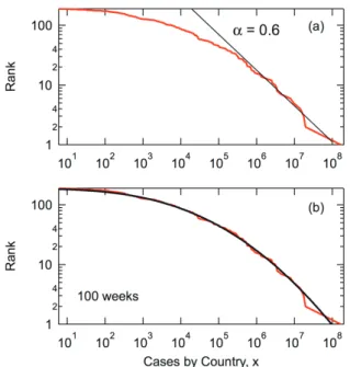
Fig. 6 shows the distribution after 100 weeks. Two characteristics are satisfied also at t = 100 weeks. The magnitude of α is about 0.6, which is smaller than that shown in Figure 5. In fact, the magnitude of α decreases

with time. Assuming a continuous distribution, the weight average of the distribution goes to infinity when the α is less than or equal to 2, and a shift to a smaller α-value implies that the situation is getting worse if the present µ distribution is preserved.

Fig. 6 MC simulation results at t = 100 weeks.

Yamamoto^[3] reported that Eq. (10) has a positive solution α, if E(lnµ) < 0 and lim

β→∞E(µ^β)= ∞. In our obtained data, E(lnµ) = 0.0523 > 0, and therefore, the distribution cannot reach the stationary state. It would be reasonable to think that if the average of µ, E(µ) is larger than unity, the number of cases continues to increase.

The present data shows that E(µ) = 1.14 > 1.

The numerical integration of Eq. (10), by using the continuous function f(µ) shown in the solid curve in Fig.

4, leads to show that the trivial solution, α = 0 is the unique solution. There is no unique positive solution.

This would be the reason for the continuous decrease of α with time, and the distribution cannot reach the stationary state.

The present MC simulation shows that the present stochastic model satisfies two notable characteristics in the ranking plot simultaneously during the transient period.

4. Suggestions to Stop the Pandemic

Assuming the present statistical model is valid and the upper tail of the ranking plot conforms to the power law,

we consider the requirements to stop the pandemic. As discussed earlier, in order to keep the weight-average cases finite, the condition, α > 2 is needed.

Fig. 7 shows the least-square fit of the µ data, by using the gamma distribution, which is represented by the following equation.

f(µ)= µ^m−1

Γ(m)η^{mexp −} µ η

⎛

⎝⎜

⎞

⎠⎟. (11)

The gamma distribution fits the data reasonably well.

The determined values of two parameters are m = 10.79 and η = 0.1003.

Fig. 7 Least-square fit of the µ data by using the gamma distribution.

With the gamma distribution, Eq. (10) is calculated to obtain the following equation.

µ^αf(µ)dµ

0

∫

Now, let us seek the values of m and η at the critical point, i.e., α = 2. Note that in order to keep the weight average of µ finite, α must be larger than 2. When α = 2, Eq. (12) reduces to:

η²(m+1)m=1. (13)

The parameter, m is represented by using the number average of µ, E(µ)=µ, as follows.

m=µ η. (14)

By substituting Eq. (14) into Eq. (13), one obtains:

η =1−µ²

µ ^{. (15)}

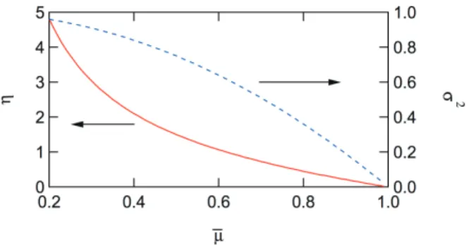
Figure 8 shows the calculated results of Eq. (15). The right axis shows the variance σ² of µ, which is given by:

σ²=mη²=ηµ (16)

40

Fig. 8 Magnitudes of η and σ² as a function of µ at the critical condition with α = 2.

As shown in Fig. 8, when the average is close to unity, the µ distribution must be quite narrow with a very small variance, σ². On the other hand, if the average is small enough, relatively broad distribution is allowed.

Fig. 9 shows the critical distribution that leads to α = 2 for µ = 0.9, 0.8 and 0.7. A common characteristic for these curves is that the probability to have the time period to make µ > 2 is rather small.

Fig. 9 Magnitudes of η and σ² as a function of µ at the critical condition with α = 2.

On the basis of the results shown in Fig. 8 and Fig. 9, to stop the pandemic, (1) the average µ must be controlled to make µ < 1, and (2) the time period for µ to be greater than 2 must be small enough. When the µ-value increases to approach 2, some strong measure to prevent the infection spread must be undertaken to make µ smaller.

Fig. 10 shows the ranking plot in Japan. The x-axis shows the number of cases by the prefecture. Because the total number of prefectures is only 47 and the data points are too small, the statistical analysis is difficult to conduct. However, the power law with about α = 0.7 –

0.8 seems to apply, which may show the statistical self-similarity with the world data, shown in Fig. 2. It would be reasonable to think that the above criteria for the prevention measure are valid also for the local area.

Fig. 10 Ranking plot by the prefectures in Japan.

5. Conclusions

The global cases of COVID-19 reported on the website of Center for Systems Science and Engineering at Johns Hopkins University^[1] are used to analyze the distribution by country. The relationship between rank and size (ranking plot) is approximately represented by the power-law distribution for the top countries.

Assuming a continuous power-law distribution, the power exponent determined from the data shows that the weight average diverges to infinity. This fact may imply the pandemic, which corresponds to the present situation in 2020.

On the other hand, the overall distribution, including the lower ranked countries, agrees reasonably with the lognormal distribution.

Here, we report two notable characteristics in the global ranking plot of COVID-19 during the year 2020:

(1) the top countries appear to follow the power-law distribution, and (2) the overall distribution could be represented by the lognormal distribution.

These two characteristics are reproduced well by the discrete-time stochastic model that employs the weekly reproduction rate µ, during the transient period. On the other hand, the present µ distribution predicts that the infection status will get worse, without changing the µ distribution.

The present µ distribution can be approximated by the gamma distribution. By assuming a gamma distribution is valid even when the infection situation changes, the required conditions to stop the pandemic are (1) the average µ must be made smaller than unity and (2) the

time period for µ > 2 must be kept small enough.

References

[1] COVID-19 Dashboard by the Center for Systems Science and Engineering at Johns Hopkins University, <https://coronavirus.jhu.edu/map.html>, (2020/04/11-11/11).

[2] H. Tobita: Mem. Fac. Eng. Univ. Fukui, 52, 37-41 (2004).

[3] K. Yamamoto: Phys. Rev. E, 89, 042115 (2014).

[4] P.J. Flory: Principles of Polymer Chemistry, Cornell University Press, Ithaca, USA (1953), Chap. 9.

[5] L. Benguigui and M. Marinov: arXiv:1507.0348 (2015).

[6] A. D. Broido and A. Clauset: Nat. Comm. 10, 1017 (2019).

42