Journal of Geophysical Research: Space Physics TECHNIQUE

TECHNIQUE

10.1002/2013JA019733

Key Points:

• A technique to estimate the plasma- spheric He+ density distribution is proposed

• The estimation is based on EUV data from the IMAGE satellite

• The uncertainty and sensitivity of the estimate are also evaluated

Correspondence to:

S. Nakano, shiny@ism.ac.jp

Citation:

Nakano, S., M.-C. Fok, P. C. Brandt, and T. Higuchi (2014), Estimation of the helium ion density distribution in the plasmasphere based on a sin- gle IMAGE/EUV image,J. Geophys.

Res. Space Physics,119, 3724–3740, doi:10.1002/2013JA019733.

Received 23 DEC 2013 Accepted 25 APR 2014

Accepted article online 30 APR 2014 Published online 19 MAY 2014

Estimation of the helium ion density distribution in the plasmasphere based on a single

IMAGE/EUV image

S. Nakano

, M.-C. Fok

, P. C. Brandt

, and T. Higuchi

1

The Institute of Statistical Mathematics, Research Organization of Information and Systems, Tachikawa, Tokyo, Japan,

2

School of Multidisciplinary Sciences, Graduate University for Advanced Studies, Hayama, Kanagawa, Japan,

Department of Meteorology, University of Reading, Reading, UK,

NASA Goddard Space Flight Center, Greenbelt, Maryland, USA,

The Johns Hopkins University Applied Physics Laboratory, Laurel, Maryland, USA

Abstract We have developed a technique by which to estimate the spatial distribution of plasmaspheric helium ions based on extreme ultraviolet (EUV) data obtained from the IMAGE satellite. The estimation is performed using a linear inversion method based on the Bayesian approach. The global imaging data from the IMAGE satellite enable us to estimate a global two-dimensional distribution of the helium ions in the plasmasphere. We applied this technique to a synthetic EUV image generated from a numerical model. This technique was confirmed to successfully reproduce the helium ion density that generated the synthetic EUV data. We also demonstrate how the proposed technique works for real data using two real EUV images.

1. Introduction

The plasmasphere is the region of cold dense plasma, which typically has a distinct outer boundary defined by a sharp density gradient referred to as the plasmapause. The averaged spatial structure of the plas- masphere has been investigated by many works. For example, Carpenter and Anderson [1992] developed an empirical model of the equatorial electron density distribution based on ISEE 1 electron density data and whistler data. Gallagher et al. [2000] modeled the ion density distribution including the composi- tion of hydrogen, helium, and oxygen ions. A number of empirical models have been proposed for the plasmapause location [Moldwin et al., 2002; O’Brien and Moldwin, 2003; Heilig and Lühr, 2013].

However, the shape of the plasmasphere is strongly influenced by the convection electric field. Since the timescale for the response to the storm time electric field is typically much shorter than the recovery of the plasmasphere to the prestorm level [e.g., Park, 1974; Obana et al., 2010], the time history of the convection electric field would control the structures of the plasmasphere. This means that a given convection electric field would not necessarily result in the plasmasphere having a unique shape. Therefore, the plasmasphere exhibits a variety of shapes as a result of the variation in the time history of the magnetospheric convection.

Global imaging observations from outside the plasmasphere provide striking evidence of the variability of the plasmasphere. In particular, the EUV imager on board the IMAGE satellite [Sandel et al., 2000] continually obtained global EUV images of the plasmasphere, which have provided important insights into the variation of the plasmasphere [e.g., Burch et al., 2001a, 2001b; Spasojevi´c et al., 2003; Goldstein et al., 2004].

The purpose of the present study is to enable the collection of information on the ion density distribution for individual events rather than simply the averaged distribution. For this purpose, we propose a linear inversion technique by which to estimate the helium ion density distribution from IMAGE/EUV data. An attempt to obtain the global helium ion density from IMAGE/EUV data was previously made by Gallagher et al. [2005]. They estimated the ion density under the assumption that the lowest L shell on the line of sight contributes most to the observed EUV intensity for each pixel. This assumption is valid if the radial density gradient is steep, as in the case at the plasmapause, but may not be valid inside the plasmasphere.

He et al. [2012] proposed an inversion method that does not require such an assumption. However, they

assumed the line of sight to be on a meridional plane and estimated the density profile for each magnetic

local time (MLT). The proposed inversion technique makes it possible to estimate the two-dimensional

distribution of helium ion density as a function of L and MLT after considering the crossing between each

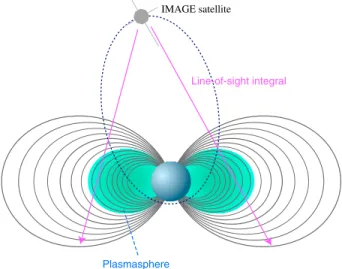
Plasmasphere

Line-of-sight integral IMAGE satellite

Figure 1. Schematic diagram of EUV observation from the IMAGE satellite.

line of sight and the meridional planes. Gurgiolo et al. [2005] also performed inversion for estimating the two-dimensional distribution of helium ion density. However, they did not take care to cope with the absence of emission from the helium ions in the Earth’s shadow, which would cause the underestimation of the density in flux tubes passing through the umbra of the Earth’s shadow. This would be inconvenient to discuss the temporal variation of the density for a given flux tube coro- tating with the Earth. The inversion technique proposed in the present paper is designed so as to produce a consistent estimate even in the umbra of the Earth.

The remainder of the present paper is organized as follows. The framework of the inversion method is explained in section 2. The proposed inversion method is validated using synthetic data in section 3. The inversion is applied to real IMAGE/EUV images, and the results are presented in section 4. Finally, a summary is presented in section 5.

2. Inversion Method

2.1. Formulation

The helium ion plasmasphere is assumed to be optically thin. Since this assumption would not be valid at low altitudes, we do not use pixels for which the lines of sight pass below an altitude of 1500 km in the esti- mation. As depicted in Figure 1, the measured signal of each pixel in an EUV image, y

, can be obtained by the line of sight integral of the helium ion density:

y

=

∫

c( 𝐫 ) n( 𝐫 ) d𝓁 + 𝜀

, (1) where n is the He

number density, c is a coefficient converting the column density into the measured EUV intensity, and 𝜀 is the observation noise. As we assume an optically thin plasmasphere, we can expect that c is constant in the sunlit plasmasphere. The value of c in the sunlit plasmasphere is given according to Gallagher et al. [2005]:

c = F

1 . 89 × 10

, (2)

where F is the 30.4 nm solar irradiance in units of photons per cm

s. We referred to the SOHO Solar EUV Monitor (SEM) data [Judge et al., 1998] for the solar EUV irradiance. In the umbra of the Earth, EUV resonant scattering is assumed to be negligible. Thus, we assume c = 0.

The goal is to estimate the spatial distribution of the He

number density, n( 𝐫 ), from the data of an EUV image taken by the IMAGE satellite. However, it is difficult to obtain a three-dimensional distribution from a two-dimensional EUV image. In order to avoid this difficulty, we assume that the density profile along a field line can be written in the following power law form as assumed in numerous other studies [e.g., Menk et al., 1999; Denton et al., 2006]:

n( 𝐫 ) = n

( 𝝆 ) ( r

r )

, (3)

where n

is the He

density at the equatorial plane, and 𝝆 is the projection of 𝐫 along the field line on the

equatorial plane. We assume the magnetic field to be a dipole. Although the power law exponent 𝛼 for

helium ions is not found in the literature, a number of studies have estimated 𝛼 for electron density or mass

density [Reinisch et al., 2009]. At high altitudes, 𝛼 is usually estimated to be approximately 1 or 2 [e.g., Denton et al., 2006], although some ground-based studies estimate that 𝛼 can be larger than 3 [e.g., Menk et al., 1999]. In the present study, we generally assume 𝛼 = 2 but also consider cases with different 𝛼 values, i.e., 𝛼 = 1 and 3. Denton et al. [2002] modeled the parameter 𝛼 as a function of the equatorial electron density.

However, if we assume 𝛼 to be a function of n

, the EUV intensity y

becomes a nonlinear function of n

which makes the problem difficult. In order to allow the use of the linear Gaussian assumption, we assume 𝛼 to have a fixed value which is independent of L and n

.

Using equation (3), equation (1) is rewritten as y

=

∫

c( 𝐫 ) n

( 𝝆 ) ( r

r )

d 𝓁 + 𝜀

= ∫

𝜂 ( 𝐫 ) n

( 𝝆 ) d 𝓁 + 𝜀

,

(4)

where we define 𝜂 as

𝜂 ( 𝐫 ) = c( 𝐫 ) ( r

r )

. (5)

We discretize the equatorial plane into a grid of cells. The He

number density n

is considered for each cell. Equation (4) can then be approximated in the following discretized form:

y

= ∑

j

𝜂

n

+ 𝜀

. (6)

We rewrite this equation in the following vector form:

𝐲 = H𝐧

+ 𝜺. (7)

The observation noise 𝜺 includes background noise, which is mainly caused by sunlight contamination.

Thus, the mean of 𝜺 is not zero, in general. We define a vector 𝐛 as the mean of 𝜺 and represent the back- ground by 𝐛 . We assume all the elements of 𝐛 take the same value and the value of an element of 𝐛 is estimated by the average of the pixels of the upper five and lower five rows for each image.

2.2. Inversion Framework

A simple method by which to estimate 𝐧

from 𝐲 is the least squares method which minimizes |𝐲 − H 𝐧

− 𝐛|

. However, the basic least squares method tends to be sensitive to observation noise. One way to reduce the influence of the observation noise is to remove the noise on the image in advance as done by Gurgiolo et al. [2005] and Gallagher and Adrian [2007]. On the other hand, we use the Bayesian approach which con- siders a priori information in the physical space to avoid the sensitivity to observation noise. This approach allows us to evaluate the uncertainty of the estimate after considering the variance of the observation noise.

The Bayesian approach considers the probability density function of 𝐧

given the observation 𝐲 , p( 𝐧

|𝐲 ), which is computed based on Bayes’ theorem:

p( 𝐧

|𝐲 ) = p( 𝐲|𝐧

)p( 𝐧

)

∫ p( 𝐲|𝐧

)p( 𝐧

) d 𝐧

. (8)

Here p( 𝐧

) is the prior distribution representing a priori information before the observation is considered, and p( 𝐲|𝐧

) is the likelihood of 𝐧

given 𝐲 representing a fitness of 𝐧

to the observation 𝐲 .

Both p( 𝐧

) and p( 𝐲|𝐧

) are assumed to be Gaussian, as follows:

p( 𝐧

) ∝ exp [

− 1

2 𝐧

P

𝐧

] , (9)

p( 𝐲|𝐧

) ∝ exp [

− 1

2 ( 𝐲 − H 𝐧

− 𝐛 )

R

( 𝐲 − H 𝐧

− 𝐛 )

] , (10)

where the superscript T indicates the transpose of the matrix. The matrix R is the covariance matrix of the

observation noise 𝜺 , and the matrix P

is the covariance matrix of the prior distribution. The method by

which to design these two covariance matrices will be discussed later.

If both p( 𝐧

) and p( 𝐲|𝐧

) are Gaussian, the posterior distribution p( 𝐧

|𝐲 ) is also a Gaussian distribution as follows:

p( 𝐧

|𝐲 )

∝ p( 𝐲|𝐧

) p( 𝐧

)

∝ exp [

− 1

2 𝐧

P

𝐧

− 1

2 ( 𝐲 − H 𝐧

− 𝐛 )

R

( 𝐲 − H 𝐧

− 𝐛 ) ]

∝ exp [

− 1

2 ( 𝐧

− 𝐧 ̄

)

P ̄

( 𝐧

− 𝐧 ̄

) ]

(11)

where 𝐧 ̄

and P ̄ are the mean vector and the covariance matrix of the posterior distribution, respectively.

The mean vector 𝐧 ̄

is given by

̄

𝐧

= (P

+ H

R

H)

H

R

( 𝐲 − 𝐛 ) . (12) The covariance matrix P ̄ is given by

P ̄ = (P

+ H

R

H)

. (13)

The posterior density p( 𝐧

|𝐲 ) is maximized at the mean 𝐧 ̄

. However, all the elements of 𝐧 ̄

, n

, are not ensured to be nonnegative even though the He

density 𝐧

must be nonnegative. Thus, we obtain an estimate of 𝐧

by maximizing p( 𝐧

|𝐲 ) subject to n

> 0 for all j.

2.3. Design of R

The matrix R gives the scale of the observation noise. The observation noise 𝜺 here represents the gen- eral discrepancy between the observation 𝐲 and the prediction from the modeled density H𝐧

+ 𝐛. The observation noise would mainly be attributed to the Poisson noise in photon counting. However, other factors can cause a discrepancy between the observation 𝐲 and the prediction. For example, although we assume a dipole magnetic field, the magnetic field around the plasmasphere is not necessarily dipole. If the assumption of a dipole magnetic field is invalid, the prediction H 𝐧

+ 𝐛 , which is derived based on the assumption of a dipole magnetic field, would contain some error. The uncertainty in the spacecraft orienta- tion might also cause a discrepancy between the observation and the prediction. The calibration error in the EUV data and the errors in the conversion function in equation (2) could also contribute to this discrepancy.

Although it is not easy to consider all of these factors, the present study assumes the Poisson noise primarily causes the discrepancy between the observation and the prediction. The effect of other factors will be discussed later.

In equation (10), the observation noise is assumed to be Gaussian. Thus, we approximate the Poisson obser- vation noise as Gaussian noise. The covariance matrix of the noise R is determined by the statistics of the EUV image itself. We assume that R is diagonal and that each diagonal element is given by the variance among the pixels in the neighborhood of each pixel. The variance is calculated by weighting the measured EUV intensity value y

according to the Euclidean distance. The weight w

is given by a Gaussian function:

w

∝ exp [

− Δ

2 𝜎

]

, (14)

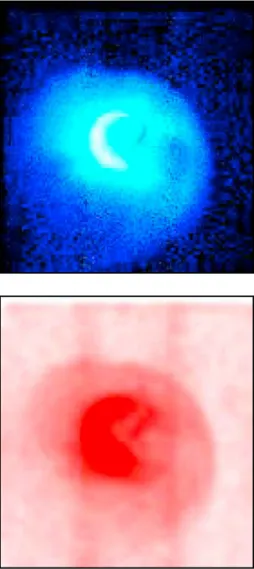
where Δ denotes the Euclidean distance between two pixels. The parameter 𝜎 is set at 2, where the unit of 𝜎 is pixels. Figure 2 shows an example of an EUV image observed from the IMAGE satellite and the amplitude (standard deviation) of the observation noise as estimated from the EUV image.

2.4. Design of P

The covariance matrix of the prior distribution P

is designed so as to ensure the smoothness of the estimated spatial distribution of ion density, 𝐧

. We set P

so as to satisfy the following relationship:

− 1

2 𝐧

P

𝐧

= − 1 2

∑

i

L

[

𝜉

( 𝜕

n

𝜕 L

)

i

+ 𝜉

( 𝜕

n

L

𝜕𝜙

)

i

]

(15)

Figure 2. (top) Example of an EUV image taken by the IMAGE satellite and (bottom) estimated amplitude of the observation noises.

where L = |𝝆| and 𝜙 is the longitude. The subscript i denotes one of the cells discretizing the equa- torial plane. The second-order spatial derivatives in equation (15) become small when the spatial distribution of n

is smooth. Thus, the prior prob- ability density in equation (9) becomes large for the smooth plasmaspheric ion distribution. Since the plasmaspheric ion density would be larger for smaller L, its spatial derivatives should accordingly be larger for smaller L. In order to take this into con- sideration, the second-order spatial derivatives are weighted by L

in equation (15). The parameters 𝜉

and 𝜉

in equation (15) represents the signifi- cance of the prior information, which determines the smoothness of the solution. If these parame- ters are taken to be too small, the prior information would virtually be ignored and the estimate would be sensitive to the observation noise. On the other hand, if the parameters are too large, most of the spatial structures could be smoothed out, and much of the information of the EUV imaging data would be ignored. Thus, 𝜉

and 𝜉

must be tuned to the appropriate value. One way to tune the parameter in the prior distribution is the empirical Bayes method [e.g., Morris, 1983] which evaluates the marginal likelihood defined as follows:

p( 𝐲|𝜉

, 𝜉

) =

∫ p( 𝐲|𝐧

, 𝜉

, 𝜉

) p( 𝐧

|𝜉

, 𝜉

) d 𝐧

. (16) The above equation evaluates 𝜉

and 𝜉

after con- sidering various probable 𝐧

. As p( 𝐲|𝐧

, 𝜉

, 𝜉

) and p( 𝐧

|𝜉

, 𝜉

) are Gaussian, p( 𝐲|𝜉

, 𝜉

) can be rewritten in the following form:

p( 𝐲|𝜉

, 𝜉

) ∝ 1

√ | HP

H

+ R | exp [

− 1

2 ( 𝐲 − 𝐛 )

(HP

H

+ R)

( 𝐲 − 𝐛 ) ]

= 1

√ | HP

H

+ R | exp [

− 1

2 ( 𝐲 − 𝐛 )

R

( 𝐲 − H 𝐧 ̄

− 𝐛 ) ]

. (17)

The parameters 𝜉

and 𝜉

are implicitly included in P

and 𝐧 ̄

in equation (17). We choose 𝜉

and 𝜉

so as to maximize p( 𝐲|𝜉 ).

3. Validation Using Synthetic Data

In order to evaluate the above inversion technique, we performed an experiment with a synthetic EUV

image. The synthetic EUV image was generated from a modeled plasmasphere obtained by a numeri-

cal model of the plasmasphere by Ober et al. [1997]. This model computes the temporal evolution of a

two-dimensional distribution of the plasmaspheric ions on the equatorial plane under a given electric

potential distribution. Here the helium ions were assumed to be distributed in the region 1 . 1 < L < 8,

which means the lower boundary is set at an altitude of 640 km. As described above, we do not use pix-

els for which the lines of sight pass below an altitude of 1500 km in the estimation. Thus, the result is not

influenced by the height of the lower boundary if the lower boundary is placed below 1500 km. Figure 3a

shows the spatial distribution of the helium ions obtained by this model under a certain condition, which

is assumed to be the truth in this experiment. Figure 3b shows the synthetic EUV image obtained from the

Figure 3. (a) Modeled distribution of helium ions for generating the synthetic EUV image, (b) synthetic image, (c) esti- mation result based on the synthetic image, and (d) the absolute values of the difference between the model and the estimate.

ion distribution in Figure 3a. This synthetic EUV image was basically generated according to equation (4), but we added weak background and Poisson noise as observation noises. The background was assumed to be 3 counts/pixel. This means the background of 3 counts/pixel was added to the EUV value obtained by equation (4) before adding the Poisson noise to obtain Figure 3b. The position of the satellite was assumed to be (x , y , z) = (0 . 21 , 3 . 08 , 6 . 67) R

in the solar magnetic coordinate system, which is the same position as the 08:32 UT on 20 June 2001, which will be examined in the next section. The parameter 𝛼 in equation (4) was assumed to be 2. Since we did not use pixels for which the lines of sight pass below an altitude of 1500 km, as described above, we did not calculate the line of sight integral for such pixels in the synthetic data. This is why the pixels around the Earth are blank in Figure 3b.

We then tried to estimate the spatial distribution of the equatorial helium ion density in Figure 3a based on the synthetic image in Figure 3b. As in the model in Figure 3a, the He

density was assumed to be dis- tributed in the region 1 . 1 < L < 8. The number of cells was 48 in the radial and azimuthal directions. In the estimation, the parameter 𝛼 in equation (3) was assumed to be 2. Figure 3c shows the estimated helium ion distribution. The equatorial helium ion density was likely to be underestimated very near the Earth. How- ever, most of the features in Figure 3a were well reproduced in Figure 3c. Figure 3d shows the absolute values of the difference between the model in Figure 3a and the estimate in Figure 3c. The wavelike pattern in Figure 3d would be an error related with a component sensitive to observation noises in the inversion.

However, the error was mostly small except for very near the Earth. Figure 4 shows the radial profiles of the estimated equatorial helium ion density on a logarithmic scale for 2 ≤ L ≤ 6. Each panel shows the profiles for a different magnetic local time (MLT): 0 MLT (top, left), 6 MLT (top, right), 12 MLT (bottom, left), and 18 MLT (bottom, right). In each panel, the gray line indicates the radial profile of the “true” helium ion density in the model results shown in Figure 3a and the thick red line indicates the estimated helium ion density profile. The two thin red dotted lines indicate the 2σ range of the posterior distribution. The blue line indi- cates the difference between the estimated density and the true density. The estimates well reproduced the true radial profiles. Since the small plume structure around 19 MLT was smoothed in the azimuthal direc- tion, the density was slightly overestimated at MLT= 18. However, the true state was within the 2σ range of the uncertainty.

Figure 3 assumed 𝛼 in equation (4) to be 2. However, the value of this parameter is normally unknown. In

order to evaluate the sensitivity of the results to the misspecification of 𝛼 , we performed the estimation

L

2 3 4 5 6

L

2 3 4 5 6

L

2 3 4 5 6

L

2 3 4 5 6

MLT=12

6 0

= T L M 0

0

= T L M

MLT=18 1e+00

5e+00 1e+01 5e+01 1e+02 5e+02 1e+03

Neq (/cc)

1e+00 5e+00 1e+01 5e+01 1e+02 5e+02 1e+03

Neq (/cc)

1e+00 5e+00 1e+01 5e+01 1e+02 5e+02 1e+03

Neq (/cc)

1e+00 5e+00 1e+01 5e+01 1e+02 5e+02 1e+03

Neq (/cc)

Figure 4. Estimation of the radial density profile with

based on the synthetic image in Figure 3b for four meridians:

(top, left) 0 MLT, (top, right) 6 MLT, (bottom, left) 12 MLT, and (bottom, right) 18 MLT. In each panel, the gray line indi- cates the true helium ion density, the thick red line indicates the estimated helium density, the two thin red dotted lines indicate the

range of the posterior distribution, and the blue line indicates the difference between the estimate and the truth.

L

2 3 4 5 6

L

2 3 4 5 6

L

2 3 4 5 6

L

2 3 4 5 6

MLT=12

6 0

= T L M 0

0

= T L M

MLT=18 1e+00

5e+00 1e+01 5e+01 1e+02 5e+02 1e+03

Neq (/cc)

1e+00 5e+00 1e+01 5e+01 1e+02 5e+02 1e+03

Neq (/cc)

1e+00 5e+00 1e+01 5e+01 1e+02 5e+02 1e+03

Neq (/cc)

1e+00 5e+00 1e+01 5e+01 1e+02 5e+02 1e+03

Neq (/cc)

Figure 5. Estimation of the radial density profile with four different

values for four meridians: (top, left) 0 MLT, (top,

right) 6 MLT, (bottom, left) 12 MLT, and (bottom, right) 18 MLT. The cyan, blue, red, and green lines indicate the estimates

with

, 1, 2, and 3, respectively. The differences from the estimate with

for the cases with

, 1, and 3 are

also plotted with the cyan, blue, and green dashed lines, respectively.

Figure 6. (a) Distribution of helium ions where artificial structures were added, (b) synthetic image generated from the helium ion distribution with the artificial structures, (c) estimation result based on the synthetic image, and (d) the absolute values of the difference between the model and the estimate.

using various values of 𝛼 for the synthetic EUV image generated using 𝛼 = 2. Figure 5 shows the radial profiles of the equatorial helium ion density estimated using four different values of 𝛼 at four different MLTs.

In each panel, the gray line indicates the radial profile of the true helium ion density shown in Figure 3a. The cyan, blue, red, and green solid lines indicate the profiles of the estimated helium ion density with 𝛼 = 0, 1, 2, and 3, respectively. The cyan, blue, and green dashed lines indicate the difference from the estimate with 𝛼 = 2 for the cases with 𝛼 = 0, 1, and 3, respectively. The estimate was not sensitive to the error of 𝛼 near the plasmapause. However, the estimate was somewhat dependent on 𝛼 in the inner part of the plasmasphere especially at 0 MLT. If 𝛼 was assumed to be 0 while the true 𝛼 value is 2, the error in the estimate was as large as a half of the true density at 0 MLT. However, at the other MLT, the error was less than 20% of the true density. For the outer region where L ≥ 3, the error was less than 10% of the truth even if 𝛼 was misspecified at 0. Thus, the error of 𝛼 is not likely to cause serious errors for the region where L ≥ 3. The sensitivity to 𝛼 at 0 MLT could be associated with the lack of the EUV emission in the umbra of the Earth. If a field line passes through the umbra of the Earth, the emission from the helium ions would be partially masked for this field line. If the density profile along a field line is not correctly given, we cannot correctly specify the relationship between the EUV emission and the helium ion density. This would cause an error in the estimated helium ion density around midnight. (Using the property whereby the emission is partially masked for a field line that passes through the umbra of the Earth, we might be able to guess the value of 𝛼 around the umbra of the Earth. Indeed, we could estimate this value for the synthetic data. At present, however, we do not necessarily attain a reasonable estimate using a real image probably due to the data quality. Thus, we do not estimate 𝛼 in the present paper. In a companion paper, 𝛼 is estimated using another approach [Nakano et al., 2014].

We also evaluated how the proposed technique works in a case when the helium ion distribution has more

complicated pattern. As shown in Figure 6a, an artificial notch around the noon and an artificial dip around

the dawn were added to the modeled plasmasphere in Figure 3a. The synthetic EUV image was then gen-

erated from the modeled plasmasphere containing these artificial structures. Figure 6b shows the synthetic

EUV image obtained from the ion distribution in Figure 6a. Figure 6c shows the helium ion distribution

estimated from this synthetic image. Most of the features in Figure 6a were well reproduced although the

estimated notch seemed to be blurred. Figure 6d shows the absolute values of the difference between the

model in Figure 6a and the estimate in Figure 6c. Errors tended to be larger in the inner part of the dayside

plasmasphere. In Figure 6a, the azimuthal gradient of the density around 12 MLT was assumed to

MLT=12

6 0

= T L M 0

0

= T L M

MLT=19

2 3 4 5 6

L

2 3 4 5 6

L

2 3 4 5 6

L

2 3 4 5 6

L 1e+00

5e+00 1e+01 5e+01 1e+02 5e+02 1e+03

Neq (/cc)

1e+00 5e+00 1e+01 5e+01 1e+02 5e+02 1e+03

Neq (/cc)

1e+00 5e+00 1e+01 5e+01 1e+02 5e+02 1e+03

Neq (/cc)

1e+00 5e+00 1e+01 5e+01 1e+02 5e+02 1e+03

Neq (/cc)

Figure 7. Estimation of the radial density profile with

based on the synthetic image in Figure 6b for four meridians:

(top, left) 0 MLT, (top, right) 6 MLT, (bottom, left) 12 MLT, and (bottom, right) 19 MLT. In each panel, the gray line indicates the true helium ion density, the thick red line indicates the estimated helium density, and the two thin red dotted lines indicate the

range of the posterior distribution, and the blue line indicates the difference between the estimate and the truth.

be steeper in the inner plasmasphere than the outer plasmasphere, and the steep gradient was smoothed in the estimate. That would be the reason of the larger errors in the inner part of the day- side plasmasphere. Figure 7 shows the radial profiles of the estimated equatorial helium ion density on a logarithmic scale for 2 ≤ L ≤ 6 for four different magnetic local times (MLTs): 0 MLT (top, left), 6 MLT (top, right), 12 MLT (bottom, left), and 19 MLT (bottom, right). Here, the profile at 19 MLT is shown instead of that at 18 MLT in order to demonstrate how well the plume structure around 19 MLT is reproduced in the estimate. The gray and red lines indicate the radial profiles of the true ion density and the estimated ion density, respectively. The thin red dotted lines indicate the 2σ range of the posterior distribution in each panel. At 12 MLT where a notch structure exists, the density was overestimated in the inner part of the plasmasphere because the notch was smoothed in the azimuthal direction. The other structures at 6 MLT and 19 MLT were successfully estimated.

As described above, the background is estimated by the average over the upper five and lower five rows of the pixels in each image. This procedure assumes that the background takes the same value over an

Figure 8. Synthetic image with background noise of 1 count/pixel generated from the helium ion distribution in Figure 6a.

entire image. However, the background is not necessarily uniform

because of the partial or nonuniform contamination from the sunlight

[e.g., Goldstein et al., 2005]. If the background is not uniform over an

entire image, the background level around the plasmasphere in the

image may not be correctly estimated, which might cause biases in the

estimation of the ion density. We then evaluate how well the ion density

can be estimated in a situation that the background level is underesti-

mated or overestimated. Figure 8 shows a synthetic EUV image which

was generated from the same helium ion distribution as Figure 6 but with

background of 1 count/pixel. We then estimated the helium ion den-

sity distribution from this synthetic image using the assumption that the

background was 3 counts/pixel, which means that the background was

2 3 4 5 6 L

2 3 4 5 6

L

2 3 4 5 6

L

2 3 4 5 6

L

MLT=12

6 0

= T L M 0

0

= T L M

MLT=19

5e+00 1e+01 5e+01 1e+02 5e+02 1e+03

Neq (/cc)

1e+00 5e+00 1e+01 5e+01 1e+02 5e+02 1e+03

Neq (/cc)

1e+00 5e+00 1e+01 5e+01 1e+02 5e+02 1e+03

Neq (/cc)

1e+00 5e+00 1e+01 5e+01 1e+02 5e+02 1e+03

Neq (/cc)

Figure 9. The radial density profile estimated from the synthetic image of Figure 8 for four meridians.

overestimated. Figure 9 shows the radial profiles of helium ion density estimated with the overestimated background. In each panel, the red and gray lines indicate the estimate and the truth, respectively. The blue lines indicate the difference between the estimate and the truth. The density was mostly well estimated.

Around the plasmapause where the true density was small, the density tended to be underestimated. This underestimation would be due to the bias caused by the misestimation of the background. Figure 10 shows a synthetic EUV image which was generated with background of 10 counts/pixel. We then estimated the helium ion density distribution from this synthetic image using the assumption that the background was 3 counts/pixel, which corresponds to a case that the background was underestimated. Figure 11 shows the radial profiles of helium ion density estimated with the underestimated background. The estimate indicated with the red lines well agreed with the true density profile indicated with the gray lines. The 2σ range of the posterior distribution indicated with the thin red dotted lines tended to be larger than that in Figure 7. The retrieval of the detailed structures such as the dip at 6 MLT and the plume at 19 MLT was also a little poorer.

However, the underestimation of the background was not likely to significantly deteriorate the estimate for most part of the plasmasphere. Even if the subtraction of the background is not sufficient, most of the resid- ual would be absorbed by the estimates for the outside of the plasmasphere. Thus, the influence from this residual would be small for the main part of the plasmasphere.

Figure 10. Synthetic image with background noise of 10 counts/pixel generated from the helium ion distribution in Figure 6a.

4. Results

In order to demonstrate how the proposed technique works, we perform the estimation of the helium ion density distribution for two real cases as follows.

4.1. Event on 20 June 2001

Figure 12a shows an EUV image taken by the IMAGE satellite at 08:32 UT

on 20 June 2001. The position of the IMAGE satellite was (x , y , z) =

(0 . 21 , 3 . 08 , 6 . 67) R

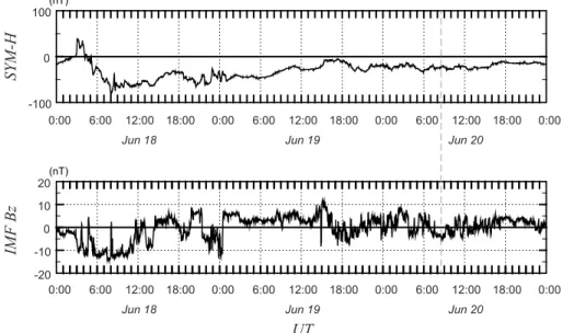
in the solar magnetic coordinate system. Figure 13

shows the SYM-H index and the north-south component of the interplan-

etary magnetic field (IMF) in GSM coordinates from 0000 UT on 18 June to

MLT=12

6 0

= T L M 0

0

= T L M

MLT=19

2 3 4 5 6

L

2 3 4 5 6

L

2 3 4 5 6

L

2 3 4 5 6

L 1e+00

5e+00 1e+01 5e+01 1e+02 5e+02 1e+03

Neq (/cc)

1e+00 5e+00 1e+01 5e+01 1e+02 5e+02 1e+03

Neq (/cc)

1e+00 5e+00 1e+01 5e+01 1e+02 5e+02 1e+03

Neq (/cc)

1e+00 5e+00 1e+01 5e+01 1e+02 5e+02 1e+03

Neq (/cc)

Figure 11. The radial density profile estimated from the synthetic image of Figure 10 for four meridians.

0000 UT on 21 June 2001. The image in Figure 12a was taken during the recovery phase of a weak magnetic storm, during which the Dst index was minimized at −61 nT at 0800 UT on 18 June which was approximately 2 days earlier. We estimated the helium ion density distribution based on the image in Figure 12a. Figure 12b shows the estimated helium ion density distribution on the equatorial plane on a log scale. As assumed in the previous section, the helium ion density was estimated for the region 1 . 1 < L < 8, which was divided into cells, and the He

density in each cell was computed using the technique described above. The num- ber of cells was again 48 in both the radial and azimuthal directions. In the estimation, the parameter 𝛼 in equation (3) was assumed to be 2. On the nightside, the plasmapause was smooth in the azimuthal direc- tion. On the dayside, the plasmapause appeared to slightly undulated although the plasmapause was not clear in the afternoon sector.

Figure 14 shows the estimated radial profile of the helium ion density at four different MLTs. In each panel,

the thick red line indicates the estimate, and the two thin dotted lines indicate the 2σ range of the posterior

distribution. The estimated helium ion density was about 10

∕cm

at L = 2, which appears to be relatively

small in comparison with the past observation by Horwitz et al. [1990] who reported the helium ion

density was around 10

∕cm

at L = 2. However, some other studies based on the IMAGE/EUV data esti-

mated the helium ion density to be around 10

∕cm

at L = 2 [Gallagher et al., 2005; Gurgiolo et al.,

2005; Galvan et al., 2008], although the estimate by Gallagher et al. was for a notch where the density

must be small. Note that the 2σ range was obtained under the given prior distribution and the given

likelihood function. As described above, we did not consider all of the factors causing the discrepancy

between 𝐲 and H 𝐧

. As such, the quantitative error might be larger than the 2σ range indicated in this

figure. At midnight and at dawn, the sharp gradients of the helium ion density corresponding to the

plasmapause were observed in the range of 4 < L < 5. At midnight, the density was depressed

around L = 2 . 8. This depression might be an artifact due to the jump in the measured signal at the

junction of the images from two of the three cameras. At noon, the plasmapause was expanded up to

around L = 5. At dusk, the plasmapause was unclear but the helium ion density decreases rather grad-

ually as the L value increased. On the duskside, since the convection electric field reduces the corotation

electric field, the drift path of the plasmaspheric ions usually expand on the duskside [e.g., Nishida, 1966].

(a)

(b)

(cm

) 10

10

10

10

Figure 12. (a) EUV image at 0832 UT on 20 June 2001.

(b) Equatorial helium ion distribution estimated from this image.

Accordingly, the plasmaspheric ions would expand outward and the gradient of the ion density would be gentle.

Although 𝛼 was assumed to be 2 in Figures 12 and 14, this assumption is not necessarily justified. We then evaluate the effects of the misspecification of 𝛼 in Figure 15, which shows the radial profiles of the equa- torial helium ion density estimated when different values were assumed for 𝛼 . As in Figure 5, the cyan, blue, red, and green lines indicate the profiles of the estimated helium ion density with 𝛼 = 0, 1, 2, and 3, respectively. The differences from the estimate with 𝛼 = 2 are also plotted with dashed lines in the respec- tive colors. Although the dependence on 𝛼 was larger than in Figure 5, the misspecification of 𝛼 appeared not to have a serious effect on the estimates.

4.2. Event on 11 August 2000

Figure 16a shows an EUV image for another case at 17:22 UT on 11 August 2000 taken from the IMAGE satellite. The position of the satellite was (x , y , z) = (−0 . 18 , 0 . 68 , 4 . 19) R

in the solar magnetic coordi- nate system. Figure 17 shows the SYM-H index and the north-south component of the IMF in GSM coor- dinates from 1200 UT on 8 August to 1200 UT on 12 August 2000. The image in Figure 16 shows the plasmasphere approximately 10 h after the main phase of a magnetic storm, in which the Dst index was minimized at −106 nT at 6 UT. At 17:22 UT, the IMF was still southward. Hence, the convection was expected to be maintained. From this image, we obtain the estimate of the helium ion distribution shown in Figure 16b. In the estimation, the parameter 𝛼 in equation (3) was again assumed to be 2. The estimate indicates that the plasmapause of the helium ion plasmasphere was distinct for almost all of the local time.

Figure 13. SYM-H index and north-south component the IMF from 0000 UT on 18 June 2001 to 0000 UT on 21 June

2001. The time at which the EUV image in Figure 12a was taken is indicated with a vertical dashed line.

2 3 4 5 6 L

2 3 4 5 6

L

2 3 4 5 6

L

2 3 4 5 6

L

MLT=12

6 0

= T L M 0

0

= T L M

MLT=18

1e+00 5e+00 1e+01 5e+01 1e+02 5e+02 1e+03

Neq (/cc)

1e+00 5e+00 1e+01 5e+01 1e+02 5e+02 1e+03

Neq (/cc)

1e+00 5e+00 1e+01 5e+01 1e+02 5e+02 1e+03

Neq (/cc)

1e+00 5e+00 1e+01 5e+01 1e+02 5e+02 1e+03

Neq (/cc)

Figure 14. Estimation of the radial density profile with

at 0832 UT on 20 June 2001 for four meridians: (top, left) 0 MLT, (top, right) 6 MLT, (bottom, left) 12 MLT, and (bottom, right) 18 MLT. In each panel, the thick red line indicates the estimated helium density, and the two thin red dotted lines indicate the

range of the posterior distribution, and the blue line indicates the difference between the estimate and the truth.

2 3 4 5 6

L

2 3 4 5 6

L

2 3 4 5 6

L

2 3 4 5 6

L

MLT=12

6 0

= T L M 0

0

= T L M

MLT=18

1e+00 5e+00 1e+01 5e+01 1e+02 5e+02 1e+03

Neq (/cc)

1e+00 5e+00 1e+01 5e+01 1e+02 5e+02 1e+03

Neq (/cc)

1e+00 5e+00 1e+01 5e+01 1e+02 5e+02 1e+03

Neq (/cc)

1e+00 5e+00 1e+01 5e+01 1e+02 5e+02 1e+03

Neq (/cc)

Figure 15. Estimation of the radial density profile at 0832 UT on 20 June 2001 for four meridians: (top, left) 0 MLT, (top,

right) 6 MLT, (bottom, left) 12 MLT, and (bottom, right) 18 MLT. The cyan, blue, red, and green lines indicate the estimates

with

, 1, 2, and 3, respectively. The differences from the estimate with

for the cases with

, 1, and 3 are

also plotted with the cyan, blue, and green dashed lines, respectively.

(a)

(b)

(cm

) 10

10

10

10

Figure 16. (a) EUV image at 1722 UT on 11 August 2000.

(b) Equatorial helium ion distribution estimated from this image.

Figure 18 shows the estimated radial profile of the helium ion density at four different MLTs. In each panel, the thick red line indicates the estimate and the two thin dotted lines indicate the 2σ range of the posterior distribution. A sharp gradient at the plasmapause was observed at all four of the MLTs.

This was in contrast with the previous case, in which the plasmapause was not clear on the duskside. This difference might be caused by the time lag from the main phase of a magnetic storm. During the storm main phase, since the strong convection electric field would intrude into the deep inner region of the mag- netosphere, the plasmasphere would shrink and the distinct plasmapause would form near the Earth. Dur- ing the recovery phase, around the plasmapause which shrank during the main phase, the corotation electric field would be dominant even on the dusk- side. Although the IMF was still southward at this time, the storm was recovering, and the convection electric field would likely decay in comparison with the main phase. Thus, the corotation field could be dominant over the convection field. If the corotation field was dominant, the plasmasphere would just corotate with the Earth and the sharp plasmapause would be maintained until refilling from the iono- sphere became effective. Figure 19 shows the radial profiles of the equatorial helium ion density estimated under four different assumed values of 𝛼 . The cyan, blue, red, and green lines indicate the profiles of the estimated helium ion density for 𝛼 = 0, 1, 2, and 3, respectively. The differences from the estimate with 𝛼 = 2 are also plotted with dashed lines in the respective colors. The estimate was not sensitive to the error of 𝛼, except for the inner region at 0 MLT. The misspecification of 𝛼 appeared not to have a serious effect on the estimates.

Figure 17. SYM-H index and north-south component the IMF from 1200 UT on 9 August 2000 to 1200 UT on 12 August

2000. The time at which the EUV image in Figure 16a was taken is indicated with a vertical dashed line.

2 3 4 5 6 L

2 3 4 5 6

L

2 3 4 5 6

L

2 3 4 5 6

L

MLT=12

6 0

= T L M 0

0

= T L M

MLT=18

1e+00 5e+00 1e+01 5e+01 1e+02 5e+02 1e+03

Neq (/cc)

1e+00 5e+00 1e+01 5e+01 1e+02 5e+02 1e+03

Neq (/cc)

1e+00 5e+00 1e+01 5e+01 1e+02 5e+02 1e+03

Neq (/cc)

1e+00 5e+00 1e+01 5e+01 1e+02 5e+02 1e+03

Neq (/cc)

Figure 18. Estimation of the radial density profile with

at 1722 UT on 11 August 2000 for four meridians: (top, left) 0 MLT, (top, right) 6 MLT, (bottom, left) 12 MLT, and (bottom, right) 18 MLT. In each panel, the thick red line indicates the estimated helium density, and the two thin red dotted lines indicate the

range of the posterior distribution, and the blue line indicates the difference between the estimate and the truth.

2 3 4 5 6

L

2 3 4 5 6

L

2 3 4 5 6

L

2 3 4 5 6

L

MLT=12

6 0

= T L M 0

0

= T L M

MLT=18

1e+00 5e+00 1e+01 5e+01 1e+02 5e+02 1e+03

Neq (/cc)

1e+00 5e+00 1e+01 5e+01 1e+02 5e+02 1e+03

Neq (/cc)

1e+00 5e+00 1e+01 5e+01 1e+02 5e+02 1e+03

Neq (/cc)

1e+00 5e+00 1e+01 5e+01 1e+02 5e+02 1e+03

Neq (/cc)

Figure 19. Estimation of the radial density profile at 1722 UT on 11 August 2000 for four meridians: (top, left) 0 MLT, (top,

right) 6 MLT, (bottom, left) 12 MLT, and (bottom, right) 18 MLT. The cyan, blue, red, and green lines indicate the estimates

with

, 1, 2, and 3, respectively. The differences from the estimate with

for the cases with

, 1, and 3 are

also plotted with the cyan, blue, and green dashed lines, respectively.

5. Summary and Discussion

We have developed a technique by which to estimate the two-dimensional distribution of helium ions in the plasmasphere using IMAGE/EUV data. In the proposed technique, a linear relationship is assumed between the EUV intensity of each pixel in an EUV image and the helium ion column abundance. The plasmaspheric helium ion density distribution is then estimated based on the Bayesian approach. The use of the Bayesian approach enables us to evaluate the uncertainty of the estimate after considering the variance of the obser- vation noise. In order to verify the performance of the proposed technique, we performed an experiment using a synthetic EUV image and confirmed that the true distribution was successfully reproduced. We also demonstrated the performance of the proposed technique for two real cases.

Estimation of the global helium ion density from IMAGE/EUV data was also attempted by some previous works. Gallagher et al. [2005] computed the “pseudodensity” based on the assumption that the lowest L shell on the line of sight contributes most to the observed EUV intensity for each pixel. However, this assumption is not necessarily valid in the inside of the plasmasphere. Gurgiolo et al. [2005] estimated the helium ion density distribution under the assumption that the ion density is constant along a magnetic field line. On the other hand, the proposed technique assumes the power law form for the density profile along a field line and performed estimation with four different values of the power law exponent.

The assumption on the density profile along a field line mainly affects the estimate of the ion density in the inner region of the plasmasphere. In order to estimate the ion density in the inner plasmasphere from an EUV image, the emission from the high-latitude part of the outer flux tube must appropriately be subtracted from a measured EUV intensity. Since the ion density at high latitudes is obtained from the equatorial den- sity and 𝛼 , the error in 𝛼 can affect the estimates for the inner plasmasphere. For the outer region where L ≥ 3, errors of the estimates were less than 10% of the truth in the situations considered in the present paper. The error in the assumption on the density profile along a field line is not likely to cause serious errors of the estimates for the outer plasmasphere.

In the present paper, the effect of the error in 𝛼 was discussed under the assumption that 𝛼 is constant for the whole inversion domain. There is no evidence to guarantee that this assumption is valid in a real situ- ation. However, even if 𝛼 is dependent on the L value, the variation of 𝛼 along the line of sight would be averaged out in the measured EUV signal. The spatial variation of 𝛼 would not enlarge the errors of the esti- mated ion density for the inner plasmasphere. Therefore, the effect of the error in 𝛼 can be satisfactorily evaluated only by considering the cases that 𝛼 is uniform for the whole domain.

The techniques proposed by the previous works did not consider the absence of emission from the helium ions in the umbra of the Earth. This would cause the underestimation of the helium ion density in flux tubes passing through the umbra of the Earth. If the ion density in the umbra of the Earth is underestimated, we cannot discuss the temporal evolution of the ion density for a given flux tube corotating with the Earth. In contrast, the proposed inversion technique takes the Earth’s shadow into consideration in estimating the ion density distribution. This allows us to consistently compare the density between the inside and the outside of the umbra of the Earth. However, in interpreting the estimation results, it should be kept in mind that the estimation for the flux tubes passing through the umbra of the Earth partially relies on the assumption on the density profile along a magnetic field line. The estimates of the helium ion density around the Earth’s shadow might be less reliable than those for the other regions.

The estimates of the helium ion density might also be affected by the error in the value of c in equation (2), which can arise due to the errors in the solar EUV flux F and the parameters in equation (2). As seen in equation (1) or (4), the observed EUV intensity has a linear relationship with c. If the EUV measurement y

is given, the estimate of the helium ion density n would be inversely proportional to c. Therefore, the shape of the estimated ion distribution would not be affected by the choice of the value of c, but the estimated density values would be changed by a factor of the inverse of c.

The assumption of a dipole magnetic field is another factor which may cause an error in the estimate. If a

magnetic field is stretched outward because of the (partial) ring current, the extent of a flux tube for a given

L value would be reduced in the north-south direction. Thus, a path of the integral of equation (4) across

each flux tube would be shorter than that in a case of a dipole magnetic field. If the ion density is estimated

by assuming a dipole magnetic field, the length of the integral path would be overestimated and the ion

density would be underestimated accordingly. According to the Tsyganenko 96 model [Tsyganenko, 1995;

Tsyganenko and Stern, 1996], if the Dst index is −80 nT, the extent of a flux tube of L = 4 in the north-south direction is reduced to be about 90% of that of the dipole field. Thus, during a moderate magnetic storm, the assumption of a dipole field can cause an underestimation of 10% of the helium ion density.

References

Burch, J. L., D. G. Mitchell, B. R. Sandel, P. C. Brandt, and M. Wüest (2001a), Global dynamics of the plasmasphere and ring current during magnetic storms,Geophys. Res. Lett.,28, 1159–1162.

Burch, J. L., et al. (2001b), Views of Earth’s magnetosphere with the IMAGE satellite,Science,291, 619–624.

Carpenter, D. L., and R. R. Anderson (1992), An ISEE/Whistler model of equatorial electron density in the magnetosphere,J. Geophys. Res., 97, 1097–1108.

Denton, R. E., J. Goldstein, and J. D. Menietti (2002), Field line dependence of magnetospheric electron density,Geophys. Res. Lett.,29(24), 2205, doi:10.1029/2002GL015963.

Denton, R. E., K. Takahashi, I. A. Galkin, P. A. Nsumei, X. Huang, B. W. Reinisch, R. R. Anderson, M. K. Sleeper, and W. J. Hughes (2006), Distribution of density along magnetospheric field lines,J. Geophys. Res.,111, A04213, doi:10.1029/2005JA011414.

Gallagher, D. L., and M. L. Adrian (2007), Two-dimensional drift velocities from the IMAGE EUV plasmaspheric imager,J. Atmos. Sol. Terr.

Phys.,69, 341–350.

Gallagher, D. L., P. D. Craven, and R. H. Comfort (2000), Global core plasma model,J. Geophys. Res.,105, 18,819–18,833.

Gallagher, D. L., M. L. Adrian, and M. W. Liemohn (2005), Origin and evolution of deep plasmaspheric notches,J. Geophys. Res.,110, A09201, doi:10.1029/2004JA010906.

Galvan, D. A., M. B. Moldwin, and B. R. Sandel (2008), Diurnal variation in plasmaspheric He⁺inferred from extreme ultraviolet images,J.

Geophys. Res.,113, A09216, doi:10.1029/2007JA013013.

Goldstein, J., B. R. Sandel, M. R. Hairston, and S. B. Mende (2004), Plasmapause undulation of 17 April 2002,Geophys. Res. Lett.,31, L15801, doi:10.1029/2004GL019959.

Goldstein, J., J. L. Burch, B. R. Sandel, S. B. Mende, P. C:son Brandt, and M. R. Hairston (2005), Coupled response of the inner magnetosphere and ionosphere on 17 April 2002,J. Geophys. Res.,110, A03205, doi:10.1029/2004JA010712.

Gurgiolo, C., B. R. Sandel, J. D. Perez, D. G. Mitchell, C. J. Pollock, and B. A. Larsen (2005), Overlap of the plasmasphere and ring current:

Relation to subauroral ionospheric heating,J. Geophys. Res.,110, A12217, doi:10.1029/2004JA010986.

He, F., X.-X. Zhang, B. Chen, and M.-C. Fok (2012), Inversion of the Earth’s plasmaspheric density distribution from EUV images with genetic algorithm,Chin. J. Geophys.,55, 1–9.

Heilig, B., and H. Lühr (2013), New plasmapause model derived from CHAMP field-aligned current signatures,Ann. Geophys.,31, 529–539.

Horwitz, J. L., R. H. Comfort, and C. R. Chappell (1990), A statistical characterization of plasmasphere density structure and boundary locations,J. Geophys. Res.,95, 7937–7947.

Judge, D. L., et al. (1998), First solar EUV irradiances obtained from SOHO by the CELIAS/SEM,Sol. Phys.,177, 161–173.

Menk, F. W., D. Orr, M. A. Clilverd, A. J. Smith, C. L. Waters, D. K. Milling, and B. J. Fraser (1999), Monitoring spatial and temporal variations in the dayside plasmasphere using geomagnetic field line resonances,J. Geophys. Res.,104, 19,955–19,969.

Moldwin, M. B., L. Downward, H. K. Rassoul, R. Amin, and R. R. Anderson (2002), A new model of the location of the plasmapause: CRRES results,J. Geophys. Res.,107(A11), 1339, doi:10.1029/2001JA009211.

Morris, C. M. (1983), Parametric empirical Bayes inference: Theory and applications,J. Am. Stat. Assoc.,78, 47–55.

Nakano, S., M.-C. Fok, P. C. Brandt, and T. Higuchi (2014), Estimation of temporal evolution of the helium plasmasphere based on a sequence of IMAGE/EUV images,J. Geophys. Res. Space Physics, doi:10.1002/2013JA019734, in press.

Nishida, A. (1966), Formation of plasmapause, or magnetospheric plasma knee, by the combined action of magnetospheric convection and plasma escape from the tail,J. Geophys. Res.,71, 5669–5679.

Obana, Y., F. W. Menk, and I. Yoshikawa (2010), Plasma refilling rates forL=2.3–3.8 flux tubes,J. Geophys. Res.,115, A03204, doi:10.1029/2009JA014191.

Ober, D. M., J. L. Horwitz, and D. L. Gallagher (1997), Formation of density troughs embedded in the outer plasmasphere by subauroral ion drift events,J. Geophys. Res.,102, 14,595–14,602.

O’Brien, T. P., and M. B. Moldwin (2003), Empirical plasmapause models from magnetic indices,Geophys. Res. Lett.,30(4), 1152, doi:10.1029/2002GL016007.

Park, C. G. (1974), Some features of plasma distribution in the plasmasphere deduced from Antarctic whistlers,J. Geophys. Res.,79, 169–173.

Reinisch, B. W., M. B. Moldwin, R. E. Denton, D. L. Gallagher, H. Matsui, V. Pierrard, and J. Tu (2009), Augmented empirical models of plasmaspheric density and electric field using IMAGE and CLUSTER data,Space Sci. Rev.,145, 231–261.

Sandel, B. R., et al. (2000), The extreme ultraviolet imager investigation for the IMAGE mission,Space Sci. Rev.,91, 197–242.

Spasojevi´c, M., J. Goldstein, D. L. Carpenter, U. S. Inan, B. R. Sandel, M. B. Moldwin, and B. W. Reinisch (2003), Global response of the plasmasphere to a geomagnetic disturbance,J. Geophys. Res.,108(A9), 1340, doi:10.1029/2003JA009987.

Tsyganenko, N. A. (1995), Modeling the Earth’s magnetospheric magnetic field confined within a realistic magnetopause,J. Geophys. Res., 100, 5599–5612.

Tsyganenko, N. A., and D. P. Stern (1996), A new-generation global magnetosphere field model, based on spacecraft magnetometer data, ISTP Newsl.,6(1), 21.

Acknowledgments

The authors would like to thank B.R.

Sandel and the University of Arizona for providing the IMAGE/EUV data. The SOHO/SEM data were provided by the Space Science Center of the University of Southern California. TheSYM-H andDstindices were provided by the World Data Center for Geomagnetism, Kyoto University. This research was supported by the Japan Society for the Promotion of Science through a Grant-in-Aid for Young Scientists (B), 24740334.

Michael Liemohn thanks Jerry Goldstein and an anonymous reviewer for their assistance in evaluating this paper.