Note on dynamically stable perturbations of parabolics

Note on dynamically stable perturbations of parabolics

Tomoki Kawahira

Nagoya University [email protected]

Abstract

In this note, we sketch some results on almost-dynamics-preserving per- turbations of rational maps with parabolic cycles.

1 Introduction with rabbits

Well known “Douady’s rabbit” has a friend called “fat rabbit” at the root of 1/3-limb of the Mandelbrot set. However the term “fat” does not sound good, so we tentatively call him “chubby rabbit”.

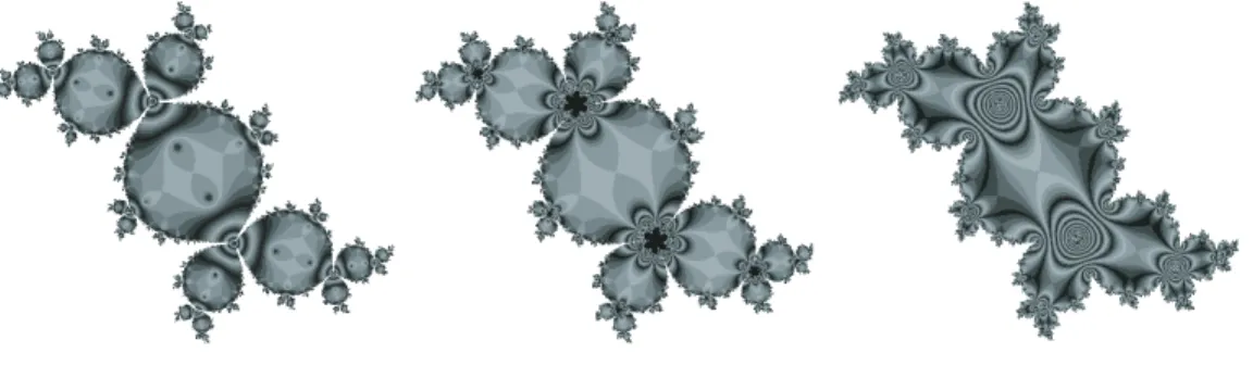
Figure 1: “plump”, “chubby”, and “overweight”.

“Chubby rabbit” has a parabolic fixed point with 3 petals and multiplier e^2πi/3. Actually there is an overweight rabbit in the main cardioid, which has an attracting fixed point with multiplier of the formre^2πi/3 (0< r <1). On the other hand, there is a little bit thinner rabbit than “chubby” near “Douady’s”, which

∗The author gave a talk on 20 February 2003 at RIMS, Kyoto. This note is written for RIMS Kokyuroku.

has a repelling fixed point with multiplier Re^2πi/3 (R > 1). So we tentatively call them “overweight rabbit” and “plump rabbit”. (I don’t know whether these terms are proper or not, though...)

The change from “chubby” to “overweight” or “plump” is parameterized by the multiplier of (α-)fixed point. They look similar when r and R are very close to 1 (Figure 1). Actually “overweight” and “plump” converge to “chubby” as r, R→1 in the Hausdorff topology. Moreover, the dynamics on the Julia sets are almost the same as we can see by observing the combinatorics of landing external rays. (By theorems in §2, we can also see that the dynamics inside the Julia sets are almost the same.)

In the general case, changes from “parabolic” to “hyperbolic” (=“attracting or repelling”), or opposite directions, are not easy as above. The difficulty comes from well-known parabolic implosion, but here we omit to deal with it. Our main question is:

For a rational map with a parabolic cycle, can we give a way to perturb its parabolic cycle into another kind of cycle without changing most part of the dynamics?

In this note, we will give a quick survey on this problem.

1.1 Preliminary

Here we list some definitions and notation.

Classes of rational maps. Letf : ˆC→Cˆ be a rational map of degree d≥2.

Here we recall some famous classes:

• f isgeometrically finite if every critical point in the Julia setJ(f) is prepe- riodic. Iff is geometrically finite, the Fatou set F(f) consists of attracting or parabolic basins.

• f is calledsubhyperboliciff is geometrically finite without parabolic cycles.

• f is called semihyperbolic if f has no recurrent critical points nor parabolic cycles in its Julia set.

In§3, we will deal with one more class of rational maps, called weakly hyper- bolic.

Perturbation. A perturbation of a rational map (resp. polynomial) f is a family of rational maps (resp. polynomials) {f :∈[0, ₀]} with some ₀ > 0 satisfying f₀ = f; degf = d; and d_ˆ(f, f) → 0 as → 0. For simplicity, we represent such a family in convergence form, f →f.

Notation.

• For a parabolic or attracting periodic point α, A(α) denotes its immediate basin.

• P(f) denotes the postcritical set of f.

• C(f) denotes the critical set of f.

2 Polynomial case: Theorems of P. Ha¨ıssinsky

In the case of polynomial, there are some results by Peter Ha¨ıssinsky. Here we sketch his sequential work related to our question. In this section we assume that f is a polynomial of degreed ≥2.

2.1 Parabolic to repelling

The first theorem is on a perturbation of direction “parabolic → repelling”.

Theorem 2.1 (Ha¨ıssinsky, [5]) Iff is geometrically finite with connected Julia set, then there exists a polynomial perturbation f →f accompanied by conjuga- cies between the actions of the Julia sets. Moreover, f are all subhyperbolic.

This theorem is extended later in §3.

Sketch of the proof. The last sentence implies that every parabolic cycle in J(f) is perturbed into a repelling cycle. We explicitly construct a rational perturbation F = f +R, where R is a rational function which takes value zero at all parabolic cycles and at finite critical orbits on J(f). (Here we allow degF ≥ degf.) Then F has cycles exactly the same places as the original parabolic cycles, but their multipliers are changed slightly by R. Here we take a properRto make them repelling. Moreover, to preserve the local degree of critical orbits on the Julia sets, we take R to have enough tangency at those points. If 1, we can take a nice topological-disk neighborhood U of J(f) such that {U, F⁻¹(U), F} is an analytic family of polynomial-like map. By straightening, we obtain a subhyperbolic perturbation f → f. Now it is known that the connected Julia sets of geometrically finite polynomials are locally connected.

Thus every external ray land on the Julia sets. To check the dynamical stability on the Julia sets, we check the stability of the ray equivalence, which is defined by shared landing points of external rays.

Goldberg-Milnor conjecture. Theorem 2.1 gives an affirmative answer to the following Goldberg-Milnor conjecture in the case of geometrically finite poly- nomials: For a polynomial f which has a parabolic cycle, there exists a small perturbation of f such that

• the immediate basin of the parabolic cycle is converted to basins of some attracting cycles; and

• the perturbed polynomial on its Julia set is topologically conjugate to the original polynomial f on J(f).

Conversely, is it possible to create parabolics from hyperbolics(=attracting or repelling)? The following results give us some partial answers.

2.2 Repelling to parabolic

Next we consider the opposite direction: “repelling → parabolic”. The second theorem is:

Theorem 2.2 (Ha¨ıssinsky, [4]) Suppose f has an attracting fixed point α and a repelling fixed point β on ∂A(α). We also add the following condition:

(B) β is accessible from A(α) and β /∈P(f)

Then there exists a polynomial g of degree d and a homeomorphism h : C → C such that

• h◦f(z) =g◦h(z) for any z ∈Cˆ−A(α);

• h(β) is a parabolic fixed point and h(A(α)) =A(h(β)); and

• h|_J(f) gives a topological conjugacy between the actions on the Julia sets.

We can remove condition (B) when f is geometrically finite. Moreover, we can modify the statement by replacing the term “fixed point” with “cycle”.

This theorem says that we can convert an attracting basin into the parabolic basin in our particular situation. The conjugacy breaks only on the immediate basin A(α), where we operate tricky surgery by means of µ-conformal map. µ- conformal map is not a quasiconformal map, though it is exponentially close to quasiconformal in some sense.

Letµ:C→D be a measurable function which satisfies Area{z ∈C:|µ(z)|>1−} ≤Ce^−η/

for someC ≥0 andη >0. Such aµis called to be in theDavid class of functions on C. Note that µ_∞ can be 1, but it is quite close to the situation µ_∞ <1 (that is,

Area{z ∈C:|µ(z)|>1−}= 0

for all 1), which will give us a quasiconformal map by solving the Beltrami equation ∂_z¯φ =µ(z)∂_zφ.

Now the main tool is:

Theorem 2.3 (David, [3]) For µ in the David class, the Beltrami equation

∂_¯zφ=µ(z)∂_zφ has a unique solution fixing 0, 1 and ∞.

We call this solution a µ-conformal map. In the proof, we will partially replace the M¨obius-hyperbolic-like dynamics nearα and β by M¨obius-parabolic-like one and will obtain a new topological dynamics F : C → C. Then F admits an invariant µwhich is in the David class, and by solving the Beltrami equation we will get the desired polynomial g.

Sketch of the proof. For simplicity we assume that A(α) contains a single critical point only. Then the dynamics in A(α) is quasiconformally conjugate to that of a Blaschke product B : D → D of the form B(z) = (z² +b)/(1 + bz²) with 0 < b < 1/3. Let Ψ :A(α)→ D be the conjugacy. By comparing with the dynamics of B_par(z) = (z²+ 1/3)/(1 +z²/3), we will find invariant “sectors” S and S_par which have similar dynamical behavior on their boundaries (Figure 2).

Indeed, there is a piecewise quasiconformal homeomorphism ψ : D → D which satisfies ψ(S) =S_par and ψ◦B =B_par◦ψ onD−S.

Figure 2: Dynamics ofB and B_par onD. The thickest curves show the boundary of invariant “sectors” S and S_par. Thinner curves show their first and second preimages.

Now we define the topological endomorphism F : C → C by F := P on C−A(α); and by F := (ψ◦Ψ)⁻¹◦B_par◦(ψ◦Ψ) onA(α). (Here we replace the hyperbolic dynamics by parabolic one.) Letσ₀ be the standard complex structure ofC, and letσ₁ := (ψ◦Ψ)^∗σ₀onA(α). We define a new almost complex structure

σ by σ := (Fⁿ)^∗(σ₁) on P⁻ⁿ(A(α)); and by σ := σ₀ elsewhere. Then we have F^∗σ =σ.

We have to use the property β /∈P(f) in (B). Actually, even if some critical orbits land on β but the other critical points do not accumulate on β, we can show that the Beltrami differential µ_σ induced by σ belongs to the David class (by taking suitableψ above). By Theorem 2.3, there exists aµ_σ-conformalφwith φ^∗σ₀ =σ a.e., and the polynomialg :=φ◦F ◦φ⁻¹ has the desired properties.

2.3 Attracting to parabolic

Next direction is “attracting → parabolic”. Before stating the third theorem, let us start with an easy example.

Pinching to be “Chubby”. We assume from now on that p and q are rela- tively prime positive integers. (That is, (p, q) = 1 where we allow p = q = 1.) Set ω:=e^2πip/q, and consider a family of quadratic polynomial

f(z) = (1−)ωz+z² : 0≤ <1 .

For fixed 0 < ₀ < 1, the dynamics of f = f₀ near the origin is conformally conjugate to T :w→(1−₀)ωw. Let Φ denote this local conjugacy. We extend it analytically to Φ :A(0)→Cby using the relationw= Φ(z) = T⁻ⁿ◦Φ◦fⁿ(z).

Now there are q symmetrically arrayed rays joining 0 and ∞ whose union is T- invariant on w-plane. By pulling them back by Φ, we can find q arcs I₁, . . . , I_q joining 0 and a repelling cycle γ₁, . . . , γ_q, which are permuted by f (That is, f(I_i) =I_j iff j ≡i+p moduloq) and disjoint from P(f) (Figure 3).

I¹ I² I³

Figure 3: Left, the Julia set for an f with p/q = 1/3. Right, the Julia set for f₀. Shadows distinguish the regions which never intersect by the iteration of f³ or f₀³.

SetI :=

jI_j. By comparing with the parabolic dynamics ofg =f₀, one can easily see thatI off plays the role of the parabolic fixed point ofg, topologically.

A priori, we can get the dynamics ofg by pinching the grand orbit ofI. What the third theorem states is that we can find a family of quasiconformal deformations {f} of f which realizes the pinching as above, and we can getg as its limit.

Theorem 2.4 (Ha¨ıssinsky, [6]) Supposef is semihyperbolic with connected Ju- lia set and an attracting fixed point α. Then the following holds:

1. For any p and q as above, there exist q arcs I₁, . . . , I_q joining α and a repelling cycle of period q permuted by f as the example above.

2. There exists a polynomialg with a parabolic fixed pointβ of multipliere^2πip/q which satisfies the following:

• There exist quasiconformal deformations {f : 0< ≤1} of f(= f₁) such that f →g is a perturbation.

• Let H denote the quasiconformal conjugacy from f to f. Then H converges uniformly as →0to the limit hwhich semiconjugates f to g.

• For y∈Cˆ, card(h⁻¹(y))≥2iff yeventually lands onβ. In particular, such an h⁻¹(y) is either I =

I_j or a connected component of its preimages.

We will see some similar results later in §3.

Idea of the proof. Let us start with a model of pinching and a caricature of quasiconformal deformation. By quasiconformal deformation, we may assume that the multiplier of α isω/2. By taking a linearizing coordinate z →w plus a covering w →ζ =w^q, the action of f on A(α) is semiconjugated to ζ → λζ on C, where λ= (ω/2)^q >0.

Now we put an almost complex structure (=a field of infinitesimal ellipses) on C as in Figure 4. By taking the angle closer to 0 and making the constant C 1, we will have a family of almost complex structures σ and associating Beltrami differentials µ which are invariant under the action of ζ → λζ. By solving the Beltrami equation ∂_ζ¯φ = µ(ζ)∂_ζφ for each , the solution φ fixing 1, λ, and ∞ gives a deformation of the quotient torus C^∗/λ to another torus with lower modulus. Then quasiconformal map φ converges compact uniformly toφ₀ :C^∗−R₋ →Cas→0, and conjugate the action ofζ →λζ toζ →ζ+1−λ.

We can pull-backσtoA(α) by (z →w→ζ)^∗ and denote it byσ. By putting (fⁿ)^∗σ on f⁻ⁿ(A(α)), and the standard complex structure elsewhere, we have an f-invariant almost complex structure and we will get a family of polynomials f in the same way as the previous theorem. This may realize the pinching “from hyperbolic to parabolic”, however, in our pulled-back situation, we are not sure

Figure 4: A caricature of the pinching. On the right half plane µ(z) = 0. For

π2 <|argz|< π−,|µ(z)|increases with dilatation ^1+|µ_1−|µ^|

| = 1 + tan²(|argz|−^π₂).

Finally|µ(z)|becomes a constant 0< C <1 elsewhere, with ^1+C_1−C

= 1+tan²(^π₂− ). Moreover, we take argµ = 0 and µ is constant along any radial lines from the origin. Hence µ is invariant under ζ →λζ.

that the limit offas→0 exists and isg as we desired. To check them, we make some effort to show that the integrating map φ of σ is equicontinuous and any subsequential limits coincide. In this technical part we use the semihyperbolicity of f. (We also use theweak hyperbolicity of f. See §3.)

2.4 Explicit construction of pinching: Tessellation

Here we present an explicit way of constructing pinching semiconjugacy. The idea is tessellation of filled Julia sets [11]. For simplicity we explain an example just by figures.

Let us consider a family of quadratic polynomials, F =

f_c(z) =z²+c:−3/4< c <0 .

Figure 5 is the pictures of tessellation for two quadratics, one is taken fromF and the other is f_−3/4. The construction of tiles are obviously based on linearizing coordinates.

Each tile has an “address”, consists of angle θ ∈ Q/Z, level n ∈ Z, and signature + or −. Addresses are organized so that the tile of address (θ, n,+) is mapped to the tile of (2θ, n+ 1,+) for example. It matches to the combinatorics of external rays, and we can precisely describe the dynamics inside the Julia set.

Now it is not difficult to construct a pinching by pasting tile-to-tile homeo- morphisms which preserve addresses. Then some of arcs (as {I_j} in the previous example f(z) = (1−)ωz+z²) are naturally pinched by continuous extentions of the tile-to-tile homeomorphisms.

Figure 5: Tessellation.

5/24

5/24

5/24

1/6

1/6 1/6

1/12

1/12 1/12

11/12 11/12 ^11/12

5/6 5/6 5/6

19/24 19/24

17/24

17/24

2/3

2/3

-1

-1 -1

-2

-2

-2

-3-2

-3

-3

-3

-3

-3 -3

-3

-2

-2 -2

0 -2

0

1 1^{2 0}

0

0 0

-4

-4 -4

-4 -4 -4

-5

-5 -5

-5

-5 -5

-5 -5 -5 -5

-5 -5 -5

-5

-5 -5

-4 -4

-4 -4

-4 -4

2

-1 -1 ^-1

2/3

7/12

7/12 7/12 5/12

5/12 5/12 1/3

1/3 1/3 7/24

7/24

17/24 19/24

7/24

+

- +

-

Figure 6: “Checkerboard” and “Zebra”, showing the structure of the addresses of tiles. “Checkerboard”, with some external rays drawn in, shows the relation between the external angles and the angles of tiles. The invariant regions colored in white and gray correspond to tiles of signature + and −respectively. “Zebra”

shows the levels of tiles. Levels get higher near the preimages of the attracting fixed point.

3 Rational case: Geometrically finite maps, etc.

Here we deal with the case of rational maps. Some results are natural general- ization of theorems in §2.

3.1 G. Cui’s plumping deformation.

G. Cui made intriguing applications of well-known Thurston rigidity to geomet- rically finite branched coverings. Here we roughly sketch some part of his work relating “parabolic → hyperbolic” perturbations. See [1] for his original, or [14]

for a survey of his entire works.

Periodic star-like graphs. Before the main statement, let us consider a ra- tional map f with an attracting cycleα of periodl. For some integersn, m with nm = l, suppose there are a repelling cycle β of period n and star-like graphs I¹, . . . , Iⁿ such that: each I^k is centered at a repelling point in β; each I^k has m feet with their toes at α; and f(I^k) =I^k+1 with superscripts modulon. We call such an I^k a repelling periodic star-like graph associated with α.

For example, readers may imagine the case of “plump rabbit”, with an invari- ant star-like graph connecting the central repelling fixed point and the attracting cycle, or the cases of its tuned quadratic polynomials (i.e. “plump rabbits” in copies of M in M). One may call the graph I =

I_j in Figure 3 an invariant attracting star-like graph centered at 0.

Plumping to be “plump”. The theorem here deals with simple plumping, which replaces parabolic cycles by repelling periodic star-like graphs without breaking the symmetry of petals, like the change of “chubby rabbit” into “plump”.

Now the statement is:

Theorem 3.1 (Cui, [1]) Letg be a geometrically finite rational map with parabolic cycles. Then there exists a subhyperbolic rational map f satisfying the following:

• There exist quasiconformal deformations {f : 0< ≤1} of f(= f₁) such that f →g is a perturbation.

• Let H denote the quasiconformal conjugacy from f to f. Then H con- verges uniformly as →0 to the limit h which semiconjugates f to g.

• For y∈Cˆ, card(h⁻¹(y))≥2 iff y eventually lands on a parabolic cycle. In particular, such an h⁻¹(y) is either a repelling periodic star-like graph or a connected component of its preimages.

Compare this with Theorem 2.4. (It was “overweight” to “chubby”.)

This theorem is stronger than Theorem 2.1, however the proof is quite different and complicated. It goes like this: Step 1, we construct a partially analytic

branched covering F by replacing all parabolics with proper repelling star-like graphs. This operation creates no Thurston obstruction. Step 2, by a result on convergence of Thurston algorithm in [2], we can find a subhyperbolic rational map f which is conjugate toF. Step 3, we construct pinching deformations{f} as in Theorem 2.4 which has the limit rational map ˆg with recreated parabolics.

Step 4, under suitable normalization of f andf, we can showg = ˆg by a rigidity result also due to [2].

Actually there is a much stronger theorem which makes Theorem 3.1 just a corollary. See Theorem D+F’+G’ in [14]. Instead of stating it in detail, we consider an example.

Example (Example 3 of [14]). Set g(z) := z(1−z²), with a parabolic at z = 0. The attracting (resp. repelling) directions lie on R (resp. iR). Let ₁ be an invariant curve in the first quadrant and L₁ the region enclosed by ₁∪ {0}, called a sepal. Fori= 2,3,and 4, let _i andL_i be the symmetric image of₁ and L₁ in the i-th quadrant. (See Figure 7.) In particular, L₁ and L₃ (resp. L₂ and L₄) are called right sepals (resp. left sepals).

L1

L2

L3 L4

Figure 7: Sepals and the filled Julia set of g.

Generalplumping is, roughly speaking, replacing a pair of right and left sepals by an invariant arc joining two fixed points. To describe possible ways of plump- ing, we consider plumping combinatorics τ as following: τ is an injective map defined on L₂, L₄, or L₂L₄; and τ|_Li (i = 2,4) is just a symmetric reflection which sends L_i toL₁ orL₃. Here is all the possible τ:

(i) τ : (L₂, L₄)→(L₁, L₃) (ii) τ : (L₂, L₄)→(L₃, L₂) (iii) τ :L₂ →L₁, τ :L₄ →L₃ (iv) τ :L₂ →L₃, τ :L₄ →L₁

There are corresponding plumpings of τ in Figure 8. Two τ’s in (iii) or (iv) give topologically the same plumpings. For example, let us pick up a plumping

Figure 8: Plumpings of type (i)–(iv), from left to right. Black, white, and gray dots show repelling, attracting, and parabolic fixed points respectively.

combinatorics τ : L₂ → L₃, that is, τ(L₂) = L₃. Consider a Riemann map φ : ˆC−L₂∪τ(L₂) → Cˆ −D which sends two prime ends at 0 to those of ±1.

Then there exists a gluing map T : ˆC−D→C which identifies the components of ∂D− {1,−1} such that T respects the holomorphic dynamics near ₂ and τ(₂) =₃.

A new plumped map F : ˆC → Cˆ will be defined basically by (φ ◦ T) ◦ g ◦(φ ◦T)⁻¹. Indeed, it is naturally defined as an analytic map except near g⁻¹(0)− {0}={1,−1}. Take a small neighborhoodU ofL₂∪τ(L₂). LetU₁ and U₋₁ be the component of g⁻¹(U) around 1 and −1. Define F on φ(U_±1) by a suitable topological map which sends ∂φ(U_±1) to φ(∂U). Then F is a partially analytic branched covering.

Cui showed that there exists a polynomial f which is conjugate to F. More generally,

Theorem 3.2 (Cui) For any plumping combinatorics τ of g above, there exists a polynomial f which is conjugate to a partially analytic map defined in a similar way as F above. Moreover, there exists a quasiconformal deformation f (0 <

≤ 1) of f = f₁ which gives a perturbation f → g, and is accompanied by (semi)conjugacies H →h as in Theorem 3.1.

See [14] for more precise statement and the proof, which deals with general geometrically finite rational maps with parabolics.

3.2 Weakly hyperbolic maps

In the case of simple plumping, Tan Lei and Ha¨ıssinsky generalized Step 3 of the proof of Theorem 3.1 to more bigger class of rational maps as following. A rational map f is weakly hyperbolic if there exist δ ≥ 1 and r > 0 with the following: For any z ∈ J(f)− {parabolics}, there exists a subsequence {n_k} of {n} such that

deg{f^nk :W_nk →B(f^nk(z), r)} ≤δ,

where B(x, r) is a spherical ball of radius r centered at x, and W_n is the com- ponent of f⁻ⁿ(B(fⁿ(z), r)) containing z. It is known that semihyperbolic or geometrically finite maps are weakly hyperbolic.

The statement is:

Theorem 3.3 (Ha¨ıssinsky and Tan, [8]) Let f be a weakly hyperbolic ratio- nal map with attracting cycles. Let I be an f-invariant collection of periodic repelling star-like graphs associated with the attracting cycles. Then there exists a rational map g with parabolic cycles which satisfies the following:

• There exist quasiconformal deformations {f : 0< ≤1} of f(= f₁) such that f →g is a perturbation.

• Let H denote the quasiconformal conjugacy from f to f. Then H con- verges uniformly as →0 to the limit h which semiconjugates f to g.

• For y∈Cˆ, card(h⁻¹(y))≥2iff y eventually lands on a new parabolic cycle created in g. In particular, such an h⁻¹(y) is either a repelling star-like graph in I or a connected component of its preimages.

The proof goes in the same way as Theorem 2.4. The difficulty is also the same, that is, we have to show the equicontinuity of H and the uniqueness of every subsequential limit. For the equicontinuity, they used a modulus-controlling inequality which is due to Cui. The uniqueness is followed by a rigidity result on weakly hyperbolic maps which is due to Ha¨ıssinsky[7].

3.3 Horocyclic perturbation of geometrically finite maps

What kind of perturbations give us dynamically stable perturbations? With the assumption of geometric finiteness, here we give a sufficient condition for this:

Theorem 3.4 (K, [9]) Let f be a geometrically finite rational map. If a per- turbation f →f is horocyclic and preserving J-critical relations of J(f) (defined below), then for 1, there exists a unique semiconjugacy h : J(f) → J(f) with the following properties:

(1) h tends to the identity. That is, sup{d_ˆ(h(x), x) :x∈J(f)} →0 (→0);

(2) If card(h⁻¹ (y))≥2for somey ∈J(f), thenyeventually lands on a parabolic cycle; and

(3) h is a homeomorphism (thus is a conjugacy) between the Julia sets if and only if none of parabolic cycles of f is perturbed into an attracting cycle.

To get a dynamically stable perturbation, we have to control two kinds of bifurcation: One is the parabolic bifurcation of course, and the other is the bifurcation of finite critical orbits on the Julia sets.

Horocyclic perturbation. Suppose that f is a rational map with parabolic cycles. We say a perturbation f →f ishorocyclic if each parabolic pointa off, with m petals and period l, satisfies the following:

(a) There is a neighborhoodD of a with local coordinates φ, φ:D→C (not necessarily conformal) such that: φ(a) = 0; φ → φ uniformly on D; and the perturbation is locally viewed as

φ◦f^lm◦φ⁻¹ (z) =λz+z^m+1+O(z^m+2)

−→ φ◦f^lm◦φ⁻¹(z) =z+z^m+1+O(z^m+2), where λ →1.

(b) If we set exp(L+iθ) :=λ, which tends to 1 as →0, then θ² =o(|L|) as L, θ→0.

Condition (a) means that the perturbation preserves the symmetry of dynam- ics near parabolics. This is not so much an essential condition but it makes the argument simpler. Condition (b) is a more crucial condition: If f has no rotation domains, then the Julia set varies continuously along horocyclic perturbations.

However, it is known that this continuity breaks when property (b) breaks.

Horocyclic perturbation was originally defined as horocyclic convergence of rational maps by C. McMullen[12,§7-9], to investigate the continuity of Hausdorff dimension of the Julia set.

J-critical relations. Letc₁, . . . , c_N be all critical points off contained inJ(f), whereN is countedwithout multiplicity. AJ-critical relation off is a set of non- negative integers (i, j, m, n) such thatf^m(c_i) =fⁿ(c_j).

We say a perturbation f →f preserves the J-critical relations of f if:

• For all i = 1, . . . , N, the maps f have critical points c_i() (may be in the Fatou set) satisfyingc_i()→c_i and deg(f, c_i()) = deg(f, c_i) as→0; and

• For eachJ-critical relation (i, j, m, n) off,fsatisfiesf^m(c_i()) =fⁿ(c_j()).

Iff is geometrically finite, then eachf is also geometrically finite.

Idea of the proof. To explain the idea, consider a perturbation of f(z) = z² into f(z) =z²+with small >0. We can make a conjugation on the Julia set in the following way: First take two attracting disks near 0 and ∞ of f. Then they are also attracting disks for f for 1, because of uniform convergence f → f. Let Ω be the compliment of these two disks, which is a closed annulus.

Set Ωⁿ := f⁻ⁿ(Ω) and Ωⁿ :=f⁻ⁿ(Ω). Then Ωⁿ⁺¹ is contained in the interior of

Ωⁿ, and the same is true for {Ωⁿ}. Set h₀ = id|_Ω. By lifting h_n to h_n+1 by the relation h_n◦f =f ◦h_n+1 forn ≥0, we obtain the following diagrams:

... ... Ω² −−−→^h2 Ω²

f



^f Ω¹ −−−→^h1 Ω¹

f



^f Ω⁰ −−−→^h0 Ω⁰

... ... Ωⁿ⁺¹ −−−→^hn+1 Ωⁿ⁺¹

f



^f Ωⁿ −−−→^hn Ωⁿ ... ...

Now one can show that h_n converges to a unique limit h on the Julia set J(f), by using the uniform expanding property of f near J(f).

Even in the case of geometrically finite f, we can take such a nice compact set Ω with J(f) ⊂ Ωⁿ⁺¹ ⊂ Ωⁿ. Indeed, we can find such an Ω of the form C−{ˆ attracting disks and petals}∪{some finite disks near critical orbits inF(f)}. We can find a similar set Ω with J(f) ⊂ Ωⁿ⁺¹ ⊂ Ωⁿ by modifying Ω near the parabolics. Then we can start lifting h₀ : Ω → Ω, which is not id|_Ω, but arbitrarily close to id|Ω by horocyclicity of f →f. Since theJ-critical relations are preserved, the lifting is not so complicated. The convergence of h_n is shown by means of a weakly expanding metric near J(f), which is compatible with the spherical metric. For the construction of this metric we again use the geometric finiteness of f.

Remark. If J(f) = ˆC, then f is postcritically finite and thus has Thurston rigidity. This implies that any perturbation f →f preserving theJ-critical rela- tions must be either a family of M¨obius conjugation or a family of quasiconformal deformation. The former happens when the associating orbifolds does not have type (2,2,2,2).

Existence of perturbation. For any geometrically finite rational map, there exists such a perturbation as in Theorem 3.4.

Theorem 3.5 (K, [10]) Letf be a geometrically finite rational map withJ(f)= Cˆ. Then there exists a horocyclic perturbation f →f which preserves J critical relations. Thus there exists a semiconjugacy as in Theorem 3.4. Moreover, one can choose the direction of the perturbation such that the parabolic cycles of f are perturbed into repelling, parabolic and attracting cycles of f in any combination.

Sketch of the proof. The proof uses quasiconformal perturbation developed by M. Shishikura[13]. First take a polynomial p(z) which vanishes at attracting

cycles, parabolic cycles, and at the finite set (C(f)∪P(f))∩J(f). (We may assume that ∞ is not periodic.) In particular, we can take p with an expansion of the form

p(z) =s(z−a) + (z−a)^M+2+· · ·+ (z−a)^k

about every parabolic point a, where s= 1, 0, or −1 depending on what kind of cycle we want, k = degp0, and M is the largest petal number of parabolics.

Letρ: [0,∞)→[0,1] be a smooth non-decreasing function such thatρ(t) = 1 at t ∈[0,1] and ρ(t) = 0 at t ∈[2,∞). In particular, we can take such a ρ with bounded derivative. Set H(z) = z +h(z)ρ(^1/k|z|). Then H : ˆC → Cˆ is a quasiconformal map if 1, and satisfies H →id and its maximum dilatation tends to 0 as →0.

Set g := f ◦H. Note that the quasiregular map g is holomorphic except V:=

z :|z|> ^−1/k

. In particular, ifais as above with periodl and multiplier λ, thena is a periodic point ofg with period l and multiplier (1 +s)^lλ. Thus it can be repelling, parabolic, or attracting depending ons = 1, 0 or−1. Moreover, g →f preserves the J-critical relations of f.

By taking a g-invariant region E and taking a M¨obius conjugacy, we may assume that g(V)⊂E if 1. Indeed, we can construct such a family of sets {E} by modifying a union of attracting disks and petals of f.

Let σ₀ denote the standard complex structure on ˆC. For 1, we put an almost complex structureσ defined by (gⁿ)^∗(σ₀) ong⁻ⁿ (E) and byσ₀ elsewhere.

Thenσisg-invariant and we can find a quasiconformal map Φsuch that Φ^∗σ₀ = σ a.e., and thus f := Φ◦g◦Φ⁻¹ is a rational map of degree d. Since Φ →id by the definition of g and the continuous dependence of Φ on its Beltrami differential, we obtain a rational perturbation f → f preserving the J-critical relations of f. By investigating local dynamics near the parabolics, we can check that f →f is horocyclic. Now we can apply Theorem 3.4.

Remarks. One can enjoy more various perturbations of parabolics by changing the polynomial p(z) above. Note that this perturbation keeps superattracting cycles, thus a polynomial is perturbed within the category of polynomials. In particular, this gives a mild generalization of Theorem 2.1.

References

[1] G. Cui. Geometrically finite rational maps with given combinatorics.

Preprint, 1997.

[2] G. Cui, Y. Jiang and D. Sullivan. Combinatorics of geometrically finite ra- tional maps. Preprint, 1996.

[3] G. David. Solutions de l’´equation de Beltrami avec µ_∞ = 1. Ann. Acad.

Sci. Fenn. Ser. A 1 Math. 13(1988), 25–70.

[4] P. Ha¨ıssinsky. Chirurgie parabolique. C. R. Acad. Sci. S´er. I. Math.

327(1998), 195–198.

[5] P. Ha¨ıssinsky. D´eformation J-´equivalence de polynˆomes g´eom´etriquement finis. Fund. Math. 163(2000), no.2, 131–141.

[6] P. Ha¨ıssinsky. Pincement de polynˆomes.Comm. Math. Helv.77(2002), 1–23.

[7] P. Ha¨ıssinsky. Rigidity and expansion for rational maps. J. London Math.

Soc., 63(2001), 128–140.

[8] P. Ha¨ıssinsky and Tan Lei. Mating of geometrically finite polynomials.

Pr´epublication Universit´e de Cergy-Pontoise, 12/2003.

[9] T. Kawahira. Semiconjugacies between the Julia sets of geometrically finite rational maps. Erg. Th. & Dyn. Sys. 23(2003), 1125–1152.

[10] T. Kawahira. Semiconjugacies between the Julia sets of geometrically finite rational maps II. Preprint, 2003.

[11] T. Kawahira. Semiconjugacies in complex dynamics with parabolic cycles.

Thesis, University of Tokyo, 2003.

[12] C. McMullen. Hausdorff dimension and conformal dynamics II: Geometri- cally finite rational maps. Comm. Math. Helv. 75(2000), no.4, 535–593 [13] M. Shishikura. On the quasiconformal surgery of rational functions. Ann.

Sci. ´Ec. Norm. Sup. 20(1987), 1–29.

[14] Tan Lei. Existence and deformations of semi-rational maps following Cui G.-Z. Manuscript, 2004.