Topology Optimization for Nonlinear Material Structures Based on Proportional Technique

Doctoral Dissertation

Shibaura Institute of Technology

Topology Optimization for

Nonlinear Material Structures

based on Proportional Technique

Topology Optimization for

Nonlinear Material Structures

based on Proportional Technique

By

Suphanut Kongwat

A dissertation submitted in partial fulfillment of the requirements for the degree of

Doctor of Philosophy in the

Department of Functional Control Systems Graduate School of Engineering and Science

I, Suphanut KONGWAT, declare that this thesis titled, “Structural Optimization of Material Nonlinearities based on Topology Design by using Proportional Technique,” and the work presented in it are my own. I confirm that:

§ This work was done wholly or mainly while in candidature for a research degree at Shibaura Institute of Technology.

§ Where any part of this thesis has previously been submitted for a degree or any other qualification at Shibaura Institute of Technology or any other institution, this has been clearly stated.

§ Where I have consulted the published work of other, this is always clearly attributed. § Where I have quoted from the work of others, the source is always given. With the

exception of such quotations, this thesis is entirely my own work. § I have acknowledged all main sources of help.

Signed: ____________________________________

“Our greatest weakness lies in giving up.

The most certain way to succeed is always to try just one more time.”

i

Acknowledgements

Firstly, I would like to express my sincere gratitude to my advisor Prof. Dr. Hiroshi Hasegawa for the continuous support of my Ph.D. study and related research, for his patience, motivation, and immense knowledge. His guidance helped me in all the time of research and writing of this thesis. I could not have imagined having a better advisor and mentor for my Ph.D. study.

Next, I would like to address my appreciation to Ministry of Education, Culture, Sports, Science and Technology on Japanese government for providing the scholarship under Monbukagakusho (MEXT) program. All transactions and financial supports are advanced to study in Doctoral course.

Last but not the least, I would like to thank my family, my parents and to my friends for providing me with unfailing support and continuous encouragement throughout my years of study and through the process of researching and writing this dissertation. This accomplishment would not have been possible without them.

Candidate Suphanut Kongwat

Thesis Advisor Prof. Dr. Hiroshi Hasegawa Program Doctor of Philosophy

Field of Study Research in Topology Design for Mechanical Engineering Department Functional Control Systems

Faculty Graduate School of Engineering and Science Academic Year 2020

Abstract

Abstract

_______________________________________________________________________________

iii

Next, a characteristic of bilinear elastoplastic material was concerned for optimizing with the static load was applied. The objective of the optimization problem is to maximize the internal energy of the structure subjected to the maximum limit of the von mises stresses to avoid failure behavior. The results from the geometrical nonlinear structure were completely different when concerned with only elasticity structure. Besides, cyclic loading was applied to the structure for topology optimization under the material characteristic of isotropic and kinematic hardening. In this case, an unloading behavior was considered during the nonlinear optimization process to acquire the optimal layout. A common weight filtering factor cannot clearly obtain a final layout from topology design when the unloading behavior was concerned. Finally, a new weight filtering factor was introduced to acquire a clear layout from nonlinear topology design without the effect of unloading behavior and possesses all requirements for optimization constraint.

Keywords: Cyclic loading, Nonlinear structure, Structural design, Topology optimization,

Acknowledgment

i

Abstract

ii

Contents

iv

List of Figures

viii

List of Tables

xii

1 Introduction

1

1.1 Background and Signification of this Research 1

1.2 Objectives 4

1.3 Scopes of this Dissertation 5

1.4 Dissertation Outline 6 1.5 Literature Review 7

2 Theoretical Issue

12

Contents

_______________________________________________________________________________

v

2.3.3 Genetic Algorithms 16

2.3.4 Level Set Method 18

2.3.5 Solid Isotropic Material with Penalization 20 2.4 Mathematical Formulations for Structural Optimization 23 2.4.1 Mass Constrained with Compliance Minimization 24 2.4.2 Stress Constrained with Mass Minimization 25

2.5 Numerical Instabilities 26

2.5.1 Local Optima 26

2.5.2 Mesh-dependence 27

2.5.3 Checkerboard 28

2.6 Crashworthiness Design for Nonlinear Material Structure 29

2.7 Nonlinear Finite Element Analysis 31

2.7.1 Nonlinear Analysis 35

2.7.2 Overview on Stress Update for Elastoplastic Materials 37

3 Opportunity for Nonlinear Design

41

3.1 Problem Signification 41

3.2 Loading Conditions for Bus Optimization 42

3.2.1 Bending Stiffness 43

3.2.2 Torsion Stiffness 43

3.2.3 Rollover Test According to ECE-R66 43

3.3 Topology Optimization of Bus Structure 45

Contents

_______________________________________________________________________________

vi

5 Model Validation

59

5.1 Optimization Model 59

5.1.1 Characteristic of Material Property 60

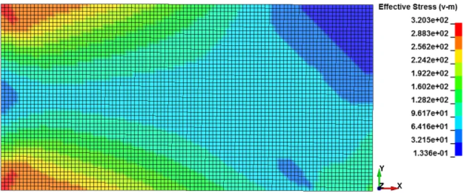
5.1.2 Analysis on Initial Design Model 61

5.2 Filtering Density 63 5.3 Optimization Problem 65 5.4 Optimization Procedure 67 5.4.1 LS-DYNA Operation 67 5.4.2 MATLAB Operation 69 5.5 Optimization Results 71

5.5.1 Linear Material Property 71

5.5.2 Nonlinear Material Property 73

5.6 Results Comparison 76

5.7 Conclusion 77

6 Optimization on Static Loading

79

6.1 Optimization Model 79

6.2 Optimization Results 82

6.2.1 Linear Material Model 82

6.2.2 Nonlinear Material Model 85

6.3 Over-relaxation Factor 88

6.3.1 Optimization Results with Over-relaxation Factor 89

6.4 Conclusion 93

7 Optimization on Cyclic Loading

95

7.1 Optimization Model 95

7.1.1 Cyclic Loading 96

7.1.2 Analysis Results on Initial Design Domain 97 7.2 Weight Filtering Factor for Optimization under Cyclic Loading 98

Contents

_______________________________________________________________________________

vii

7.4 Optimization Results 100

7.3.1 Bilinear Elastoplastic Material 101

7.3.2 Isotropic and Kinematic Hardening Material 108

7.5 Conclusion 116

8 Summary and Recommendations

118

8.1 Summary 118

8.1.1 Major Contributions 120

8.2 Future Recommendations 121

References

123

1.1 Types and overview of structural optimization 2 1.2 A load-displacement curve of geometrically nonlinear structure 10 2.1 Discretization on design area by using finite element 14

2.2 Rectangular microstructure 15

2.3 Overall process of the genetic algorithms 17

2.4 Crossover of the chromosomes based on the genetic algorithm 18 2.5 Relationship between the relative stiffness and the volume density 21 2.6 Microstructures of material and void realizing the material properties 21

of the SIMP model with the penalization factor equal to 3

2.7 Local and global optima 26

2.8 Optimal solutions from the SIMP method 27

2.9 An example of the checkerboard pattern 28

2.10 Area under force-displacement diagram represents the energy absorption 31

2.11 Classification on analyses 34

2.12 Plastic behavior is demonstrated from the uniaxial test 38 2.13 Yield surface in principal stress space in pressure independent 38

2.14 Plastic strain is normal to the yield surface 39

3.1 Bus accident in United States of America on 2012 42

3.2 Specification for bus rollover test according to ECE-R66 44

3.3 Specification of residual space 44

List of Figures

_______________________________________________________________________________

ix

3.5 The first topology optimization loop with the results of pillar 46

3.6 Optimization results for side structure 47

3.7 Optimization results for roof and floor structures 47 3.8 Proper model of bus structure from topology optimization 47

3.9 Rollover analysis of the preliminary bus frame 48

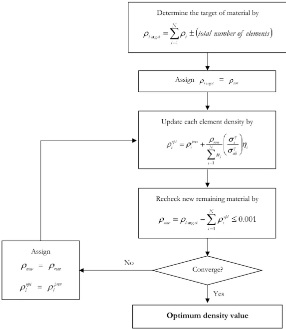
4.1 Overall process for structural topology optimization 53

4.2 Investigation of the target material amount 54

4.3 Step-by-step of the proportional topology optimization process 57

5.1 Design domain for verification model 60

5.2 Finite element model of the initial design domain 60

5.3 Bilinear elastoplastic material properties 61

5.4 Deformation in the vertical direction of the initial design model 62 5.5 Von Mises stress in the vertical direction of the initial design model 62

5.6 Internal energy of the initial design domain 63

5.7 Element pattern by one-node connectivity for checkerboarding 63

5.8 Prescribed filtering radius 65

5.9 Overview the topology optimization process 70

5.10 Characteristic of elastic material 71

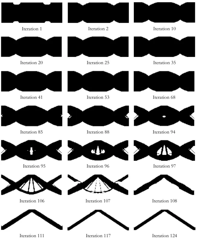
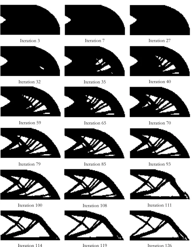
5.11 Iterative material distribution for the validation process based on 72 linear material structure

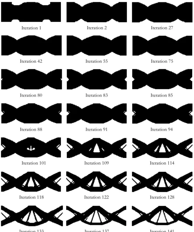
5.12 Final layout on linear structure for the verification model 73 5.13 Stress distribution of the final layout for the linear verification model 73 5.14 Iterative material distribution for the validation process based on 74

nonlinear material structure

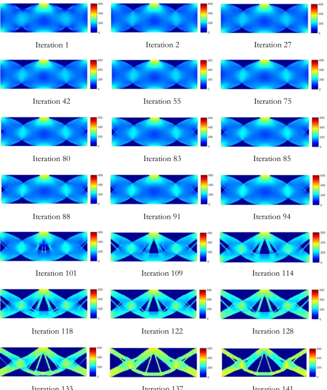
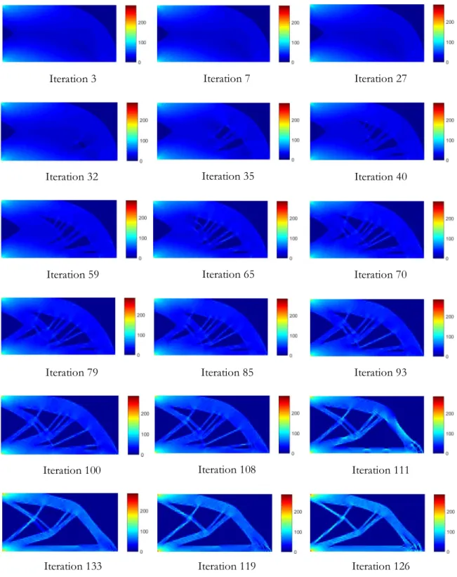
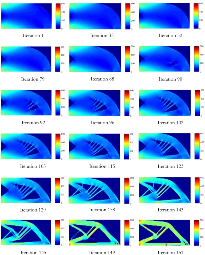
5.15 Iterative stress distribution for the validation process based on 75 nonlinear material structure

List of Figures

_______________________________________________________________________________

x

6.3 Vertical displacement of the initial design model on static loading 81 6.4 Stress distribution of the initial design model on static loading 82 6.5 Iterative material distribution for static loading on linear analysis 83 6.6 Iterative stress distribution for static loading on linear analysis 84

6.7 Maximum stress during the optimization process 85

6.8 Iterative material distribution for static loading on nonlinear analysis 86 6.9 Iterative stress distribution for static loading on nonlinear analysis 87 6.10 Histories on topology optimization with the over-relaxation factor 89 6.11 Comparisons of the final layout for over-relaxation factor 91 6.12 Comparisons of the stress distribution for over-relaxation factor 92 6.13 Comparisons of the internal energy for over-relaxation factor 92 6.14 Comparisons of the maximum stress during the optimization process 93

for over-relaxation factor

7.1 Cyclic loading behavior 96

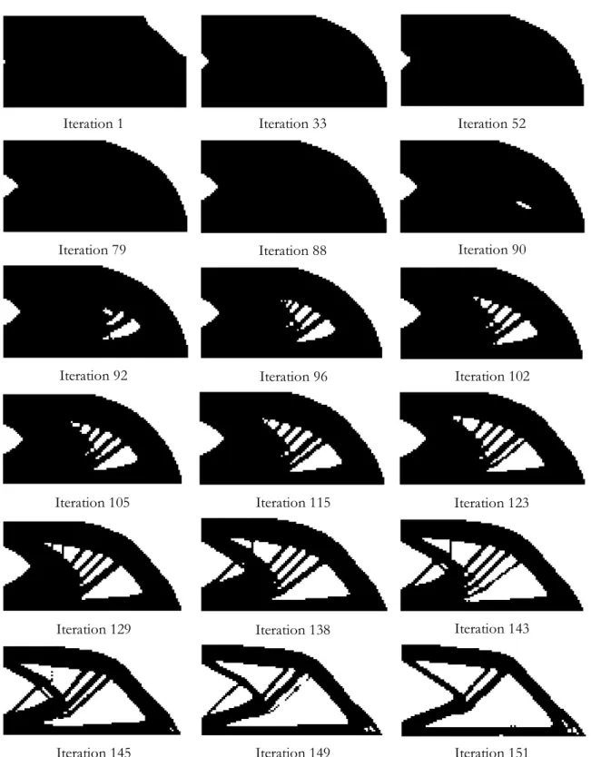
7.2 Maximum stress based on the static and cyclic load cases 97 7.3 Isotropic and kinematic hardening material properties 99 7.4 Iterative material distribution on bilinear elastoplastic material with 102

cyclic loading of Model A

7.5 Iterative stress distribution on bilinear elastoplastic material with 102 cyclic loading of Model A

7.6 Iterative material distribution on bilinear elastoplastic material with 103 cyclic loading of Model B

7.7 Iterative stress distribution on bilinear elastoplastic material with 103 cyclic loading of Model B

7.8 Iterative material distribution on bilinear elastoplastic material with 104 cyclic loading of Model C

7.9 Iterative stress distribution on bilinear elastoplastic material with 105 cyclic loading of Model C

List of Figures

_______________________________________________________________________________

xi

7.11 Internal energy of the three models during the optimization process 107 based on the bilinear elastoplastic material

7.12 Iterative material distribution on isotropic and kinematic hardening 109 material with cyclic loading of Model A

7.13 Iterative stress distribution on isotropic and kinematic hardening 109 material with cyclic loading of Model A

7.14 Iterative material distribution on isotropic and kinematic hardening 110 material with cyclic loading of Model B

7.15 Iterative stress distribution on isotropic and kinematic hardening 110 material with cyclic loading of Model B

7.16 Iterative material distribution on isotropic and kinematic hardening 111 material with cyclic loading of Model C

7.17 Iterative stress distribution on isotropic and kinematic hardening 112 material with cyclic loading of Model C

7.18 Internal energy of the three models during the optimization process 113 based on the isotropic and kinematic hardening material

7.19 Maximum stress of three models during optimization process 115 based on isotropic and kinematic hardening material

7.20 Stress fluctuation during the optimization process based isotropic 116 and kinematic hardening material

2.1 Classification of nonlinear analyses 33

5.1 Material properties for void material 68

5.2 Coding structure for LS-PrePost SCL 68

5.3 Overview process for coding on MATLAB 69

6.1 Comparisons on optimal layout based on the over-relaxation factor 90 7.1 The optimal layout of structure based on the bilinear elastoplastic model 108 7.2 The optimal layout of structure based on the isotropic and kinematic 114

I

NTRODUCTION

2

structural optimization and usually applies to be the preliminary design process. Purpose of the topology optimization is to find an optimum material distribution inside the design domain by assigning the element density of each element to be the design variable. For topology optimization, the result will be shown a necessary area of material which should remain (solid element) or the useless area which should remove (void element). As mentioned above, only topology optimization has to determine the optimum distribution of material by not considering the layout of the initial design domain.

(a) Size optimization

(b) Shape optimization

(c) Topology optimization

Figure 1.1 Types and overview of structural optimization [1].

3

the optimization problems. Therefore, a number of optimization methods have been developed for solving various optimization problems in which the optimal seeking method is also known as a mathematical programming technique. For the topology optimization, there are also many optimization algorithms are employed for investigating the best result. In order to acquire the final layout, the optimization algorithms are integrated with a numerical analysis such as the meshfree method or finite element method (FEM).

The topology optimization always concerns for a linear problem or elastic material properties in which the structure can recover after deformed. However, when the external load is applied to the structure and causes large deformation, this case is necessary to consider the problem into nonlinearity. There are three categories for consideration the nonlinearities for mechanical structure: contact or friction problems, kinematics problems (large displacement, large rotation, etc.), and material nonlinearities problems. The technique for seeking the optimal layout under the nonlinear structure might be different and depended on the application of each problem. So, a methodology, algorithm, and the layout for topology optimization under nonlinear problems are also a difference from the elasticity.

4

To achieve the problem of nonlinear topology optimization, this dissertation aims to propose the proportional method for updating the element density during topology optimization under fully nonlinear analysis. The proportional algorithm is implemented by including the fully stress design criteria for topology design as a factor of the update function. The optimization method performs with Solid Isotropic Material with Penalization (SIMP) approach according to an application of crashworthiness design. A study on static and cyclic loads were conducted to acquire the optimal layout based on structural topology design in this dissertation. The optimal layout should clearly obtain for nonlinear topology optimization and different from the elastic behavior. A new weight filtering factor for cyclic loading of topology design also proposed in this research. Finally, numerical examples based on the nonlinear design with the proportional technique are also examined.

1.2 Objectives

1.2.1 Optimize a mechanical structure under topology optimization by concerning nonlinear problem based on nonlinear material geometries:

This dissertation aims to optimize the mechanical structure by using the topology optimization method under nonlinear behavior. A nonlinear analysis and nonlinear material geometries will be concerned during the optimization procedure. Therefore, the permanent deformation of the structure will be included for acquiring the final layout.

1.2.2 Implement an update function for nonlinear structural design for updating an element density of each design variable:

5

1.2.3 Design the structure based on topology technique with a static and cyclic loads are applied as an external load:

An external load is applied based on the characteristic of static and cyclic loads to the structure by concerning an unloading effect. For the cyclic load, an unloading point affects structural behavior when the permanent deformation is concerned. Therefore, an optimization procedure and structural behavior between static and cyclic load will be different and affects the final layout.

1.2.4 Propose a new weight filtering equation for designing the structure under topology optimization when unloading behavior is concerned:

To avoid a checkboard pattern problem during the optimization procedure, the weight filtering equation is used for investigating a neighbor element connectivity. Thus, the efficient filtering factor indicates the good final layout after topology optimization and performs a numerical analysis for all procedures.

1.3 Scopes of the Dissertation

1.3.1 Optimal layouts of a prescribed design domain are determined by investigating an element density of each design variable based on topology optimization procedure as the preliminary design process.

1.3.2 Nonlinear analysis is considered on the category of material characteristic of nonlinear behavior on two types: bilinear elastoplastic material property and isotropic and kinematic hardening material property.

6

1.3.4 Numerical examples are focused on shell element model (2D element) with concerned the material distribution for the optimization process on two-dimensional only. Shear stress, which causes along to direction of load, is assumed to be small and neglect in this study.

1.4 Dissertation Outline

This dissertation aims to present the methodology for nonlinear topology optimization under material nonlinearities. Therefore, the structure of this dissertation is organized as follows:

Chapter 1 introduced the background and signification of this study. The objectives and scopes was set to achieve the target of the current work. Moreover, related studies also reviewed for concerning on method and procedure of this research.

Chapter 2 explains on the theoretical issue of structural optimization and nonlinear finite element analysis. A general formulation of the optimization process and complements of the topology optimization problem are described to conduct the complete optimization problem before optimizing the structure. And the problem of nonlinear topology design is also explained in this chapter.

Chapter 3 describes on opportunities to apply the nonlinear topology optimization for application of crashworthiness design. A fully dynamic analysis by finite element always uses to investigate the structural strength and occupant’s safety. Therefore, optimization on dynamic problem by finite element is a one choice for engineering design for automotive manufacturer.

Chapter 4 proposes a new proportional algorithm for updating element densities during topology optimization. The updated procedure of the proportional technique will display in this chapter until it obtains the optimal density of each design variable.

7

topology design. The optimal layout is compared with the results on the gradient approach to investigate an effective on this algorithm and procedure.

Chapter 6 investigates an optimal layout for nonlinear topology optimization by focusing on static analysis with the constant load. Over-relaxation factor uses for reducing a computation cost during the optimization procedure are also examined. The layout from the nonlinear analysis is compared with the elastic material property.

Chapter 7 shows an optimization process when the cyclic loading is applied. The optimal layout cannot acquire with a common weight filtering factor. So, the new weight filtering factor is proposed in this chapter for nonlinear topology optimization under cyclic loading.

Chapter 8 is a final chapter in this dissertation and concludes the study along with discussion regarding future works opportunities in this research.

1.5 Literature Review

Structural optimization is a process to design a suitable condition corresponding to each problem. There are three categories for structural optimization: size optimization, shape optimization, and topology optimization. Size and shape optimization is used for optimizing the structure when their initial design already obtained. On the other hand, the topology optimization applies to determine a preliminary layout from unknown shape and size of that structure. Therefore, topology optimization is the most complicated method and technique for the structural design process.

8

with Penalization (SIMP) approach and employed to optimize the structure under the two-dimensional problem [3]. Likewise, a three-two-dimensional problem was also determined the final layout based on the regularized SIMP interpolation approach under stiffness and volume conditions [4]. The level set approach is one technique to acquire the optimal layout by using iso-surface of the level set function. A two-dimensional structure was optimized based on the level set method and combined with discrete function [5] and the reaction-diffusion equation [6] under linear problems. Moreover, the immersed interface method [7] and fictitious interface energy [8] also proposed for combining with the level set method for solving the topology optimization problem. The combination of the topological level set method, augmented Lagrangian algorithm, and assembly-free deflated finite element was suggested for solving multi-constraint on a three-dimensional topology problem [9]. As mentioned above, both SIMP and level set approaches are common schemes for seeking the optimal layout of the structure. Furthermore, a discrete method, which is a hard-killed approach (indicates only presence or absence materials), is also applied for finding the optimal layout under topology optimization. A genetic algorithm [10] or Ant colony optimization [11] were also adopted and acquired the suitable structure under linear problem. A commercial software was implemented for optimizing the structure under topology and multidisciplinary design [12, 13], and used that design process for application of engineering to design the vehicle structure based on the results from finite element analysis [14, 15]. Most studies usually seek a suitable layout based on maximizing stiffness under mass constraint and volume minimization under displacement constraint. However, both cases can generate the final layout-based material distribution, which sustains the best way for the applied load under user-defined boundary conditions [16].

9

mathematical programming which proposed to solve topology optimization under large displacement problem [19]. All subproblems of the SLPL method were converted into linear programming to speed up the algorithm on the nonlinear design. Nonlinear programming has investigated performance on the level set approach for topology optimization with methods of moving asymptotes (MMA) and a globally convergent modification under nonlinear problems [20]. Kreisselmeier-Steinhauser (KS) function was maximized for solving the geometrically nonlinear structure by using the level set method under volume constraint [21]. The results were effectively compared to the final layout from other criteria of stiffness problems. These problems were assumed for the large displacement of the structure under linear analysis for nonlinear behavior. A mesh-free particle technique was also proposed to determine the optimal structure under the geometrical nonlinearity problem by using the level set approach [22]. Reduced Order Model (ROM) was introduced to alleviate the heavy computational cost of nonlinear topology optimization [23]. The ROM can reduce a multiscale model for macroscopic structural design on stiffness problem using discrete level-set approach. A nature-inspired method, which imitates an animal behavior in nature, was a one optimization technique and developed for solving the problem on nonlinear topology optimization. Artificial bee colony algorithm (ABCA) was used with a rank-based method to improve the candidate solutions and results [24], while a modified ant colony optimization (ACO) was developed to obtain a stable robust design [25]. Both ABCA and ACO were adopted to optimize the structure under structural stiffness problems. Most studies focused on the stiffness of structure on nonlinear geometry due to compliance of the structure is not equal to two times of complementary work and strain energy [20], along to the typical of load-displacement cure of nonlinear structure (figure 1.2). Therefore, different results may be obtained if a different function is used in optimization process under geometrical nonlinearity.

10

problem, a meshless method was employed to resolve the nonlinear topology problem, which formulated with the element-free Galerkin (EFG) method [26]. Element connectivity parameterization (ECP) was introduced to resolve an analytic sensitivity problem on nonlinear topology optimization when the commercial nonlinear finite element code is used for the two-dimensional problem [27]. In the same way as a three-dimensional problem, an internal ECP (I-ECP) also developed to substantially enhance computational efficiency on topology optimization under nonlinear material behaviors [28].

Figure 1.2 A load-displacement curve of geometrically nonlinear structure.

A sensitivity analysis is commonly required through the optimization process under nonlinear topology design. The sensitivities of the objective functions were derived and conformed to the adjoint method [18, 29, 30]. On the other hand, a non-sensitivity approach also proposed as a proportional method for optimizing the structure under the topology problem. Mechanical structures were optimized by manipulating the proportional method [31], and the results were significant compared to each optimization function. The proportional method was adopted to the robust topology design for solving the loading uncertainty problem [32]. Multi-material interpolation problem was solved by applying the proportional technique with the SIMP approach and effectively realize the polarization of

11

the intermediate-density elements [33]. Almost researchers concerned about the stress ratio at the current state of each element and on the summation of stress on the design area to be the update function through the proportional method. Furthermore, the optimization problem was also considered to a linear problem.

T

HEORETICAL ISSUE

This chapter lectures on general technique for structural optimization, especially, methods for topology optimization. An algorithm of Solid Isotropic Material with Penalization (SIMP) approach which employed for the optimization procedure in this research. The procedure of nonlinear finite element analysis is also explained in this chapter.

2.1 Size Optimization

13

condition. Figure 1.1a showed an example of size optimization by adjusting the diameter of structural elements.

2.2 Shape Optimization

This technique is similar to the size optimization because the preliminary design, such as number of holes, beams, etc., of the structure, needs to be decided before the shape optimization is applied to that structure. The design variables of this technique can be thickness distribution along with structural members, diameter of holes, radius of fillets, or any other measure inside the structural domain. Results from the shape optimization will not show a new hole, split the design domain, or new structural layout. However, an optimal dimension of each design variable (as mentioned above) will be resulted (as shown in figure 1.1b). To update the shape inside the design domain, the Perturbation vector approach [1] is a common method to employ with the shape optimization to change the shape to the discretized the finite element model.

2.3 Topology Optimization

The first step and most general process for structural design is the topology optimization technique. To design the structure based on size and shape optimization, the preliminary layout of the structure can be acquired by employing the topology technique for investigating an optimal layout, the number of holes, the direction of filet, etc., of the preferred design area under each loading condition. The topology optimization will result in optimal material distribution by deciding which area should be remain or remove areas (as in figure 1.1c).

14

of the design variable. The process of topology optimization will find the optimal location for overall design variables by identifying the number of 1 or 0 of each element for representing a solid or void element, respectively. The topology problem can be classified into two types: hard-killed and soft-killed problems. The hard-killed problem indicates a value of design variables into 0 or 1 only, while the value of each design variable during the optimization process can be continuous from 0 to 1 in case of the soft-killed problem.

Figure 2.1 Discretization on design area by using finite element.

Many methods were proposed in order to update the design variables on the topology optimization process, or some methods also can be selected for the new design variables randomly. Thus, a selection and verification of procedure for updating the design variable based on topology design are important because the results may differ due to local or global optima. Moreover, the scheme for updating the design variable will affect the number of iterations until the global optimum is obtained. The common approaches for the topology optimization based on continuum structure are described in the following sub-section.

2.3.1 Homogenization Method

The effective material properties of the equivalent homogenized domain in a physical can be found by applying the homogenization method which it is an emergent by mathematical theory [37, 38]. This approach can be used in topology optimization as the structure to be optimized can be considered as a composite consisting of material and void. Bendsoe and Kikuchi [39] proposed the application of topology optimization based on the homogenization method by deriving the effective material properties for porous finite elements. Figure 2.2 showed the assumption of holes by rectangular shape, the porous

- Design area -

Design area discretized

15

finite elements can be formulated based on three parameters of the rectangular geometrical of sizes and direction which represented by a(x), b(x) and , respectively. All parameters were assigned to design variables and the density were varying from 0-1 on the porous region. The homogenization method has a rigorous theoretical basis which can provide a mathematical bound to the theoretical performance of the structures and faster to converge. On the other hand, a determination and evaluation of the optimal microstructures is cumbersome, and the solutions cannot be built directly since no definite length scale is associated with the microstructure [2].

Figure 2.2 Rectangular microstructure [40].

2.3.2 Evolutionary Structural Optimization

Evolutionary structural optimization (ESO) is an optimization method that combines heuristic methods and gradient based approaches [41]. The ESO scheme is classified into the soft-killed method for topology optimization due to the varying density value of each design variable. This method started by finding the optimal solution from a bigger design space, which expected to obtain the final layout by removing an inefficient stress material. The ESO method was initially introduced an evolutional algorithm with two forms. The first form allows removal of the material from the surface or part; this produces a Min-Max situation where the maximum surface stress is reduced to a minimum. The

16

second form was the under-stressed material could be removed from anywhere in the allowable design space, and with compensation for checker-boarding; this produces an optimum topology under the prescribed environments. On the contrary, the element of the discretized design domain can be added to the structure where they are needed by using an additive evolutionary structural optimization (AESO) [42]. The AESO method was the opposite procedure from the original ESO, while the evolutionary process is similar. Moreover, a bi-directional evolutionary structural optimization (BESO) [42-44] was presented by combining the AESO and ESO to improve results and convergence time of both AESO and ESO. The BESO was an effective method for removing an unwanted design element in which stress was not affecting the design criteria from the structure iteratively and added the efficient material to the design area where the high stress occurred simultaneously.

The advantages of the ESO, AESO, and BESO are a reasonable computational cost and high quality of the solutions after the optimization process. The optimization algorithms of these schemes are also easy to implement and understand [45]. However, the evolutional methods are complicated to apply with the optimization problem for other constraints, such as displacement constraint, or multiple loading conditions. An investigation of the evolutionary methods [46] showed the BESO method resulted in a local optimum rather than non-local optimum, while the same results can be achieved by employing the density method, only using the high value of penalization factor and changing the initial density of the design domain.

2.3.3 Genetic Algorithms

17

generation from the parent design. The child generation mutates until it reaches the limits of a random number, which expected to be a higher quality of the parent design and replaces the parent generation. This evolutionary process is repeated until the optimal design is reached [49, 50].

Figure 2.3 Overall process of the genetic algorithms (a) a chromosome

(b) chromosome substitution in mesh (c) layout generation from the chromosome (d) an optimal layout from topology optimization.

18

variables are substituted into the mesh for representing the structural layout with solid (equal to 1) and void (equal to 0) elements (figure 2.3b and 2.3c). The optimal layout (figure 2.3d) will obtain after a connectivity analysis, which expecting the result to void all unconnected elements [51, 52]. A single point crossover for the chromosome is the most basic method by selecting and the segments of the code after that are swapped randomly (figure 2.4). By the way, there are other methods that also possible for crossover the chromosome during the optimization procedure [52].

The genetic algorithms have disadvantaged by the high computational cost due to a large number of design variables and function evaluations. So, this method is suitable for optimizing the problems with little knowledge about the nature of the design domain [53]. However, the genetic algorithms are less chance to meet the local optimum by comparing to the gradient based methods.

Figure 2.4 Crossover of the chromosomes based on the genetic algorithm.

2.3.4 Level Set Method

19

layout during the optimization process [55-60]. Thus, the level set function is necessary for the level set method because it uses to define the interface between material phases implicitly.

The two-phase material-void problem is the simplest for the level set method and often used for treading the case in structural optimization. The design domain , void area , and the interface area usually relate to the level set function as follows:

(2.1)

where X is a point of design domain and c is a constant value [55, 58]. For the level set function, most studied have been concerned the concerned the constant value (c) of equation 2.1 equal to zero. Changing of the level set function adjusts the level of design domain and possibility to topology the design material during the optimization process. To change the level set function, the Hamilton-Jacobi equation was frequently proposed for the level set method as follows:

(2.2)

where vn(x) is a normal velocity by obtaining from the sensitivity analysis of the objective

function with respect to the boundary variation. Thus, an updating of the level set function by moving the boundary along the normal direction is necessary to solve the equation 2.1. Moreover, the level set method requires a regularization technique to obtain a well-posted optimization problem to remove numerical instabilities and improve convergence behavior. The level set method is close to the shape optimization because the shape-sensitivity analysis is possible to apply with the level set method and alter only the boundaries of the

20

design domain [55, 56]. In the other hand, regularization technique [8] were also used for controlling the geometrical properties of the final design.

2.3.5 Solid Isotropic Material with Penalization

The Solid Isotropic Material with Penalization (SIMP) was introduced to the topology optimization process shortly after the homogenization method has been proposed. The SIMP or power-law approach suggested to be an easy optimization algorithm but can be artificial for reducing the complexity of the homogenization approach. Furthermore, the SIMP method also aimed to improve the convergence of the solutions by relaxing to the continuous problem, available the results vary in a range of 0 and 1 (not only 0 and 1) or material density from 0% to 100%, respectively.

A small lower bound of the element density is usually imposed as for avoiding a singular finite element method problem. The relationship between element density and Young’s modulus in the equilibrium calculation can be shown as follows:

(2.3)

where E is the elastic properties, p is the penalization factor that is always greater than 1 and E0 is initial stiffness matrix. The relationship between the relative stiffness (E/E0) and

the volume density or element density ( ) was shown in figure 2.5 with various the penalization factor, and it can be illustrated for recommendation the suitable value of the penalization factor. There were some studies applied the penalization factor (p) equal to 1, that optimization problems corresponds to the so-called “variable-thickness-sheet”. The variable-thickness-sheet problems usually are the convex problem with the unique solution [61, 62]. Selecting the penalization factor (p) too law or too high effects to the too much gray scale or too fast convergence of the optimal layout. Therefore, the recommendation of the penalization factor (p) is equate to 3 [63] as the magic number to ensure physical realizability of elements with intermediate densities. Microstructures of material and void

21

realizing the material properties of the SIMP model was shown in figure 2.6 by applying 3 for the penalization factor (p).

Figure 2.5 Relationship between the relative stiffness and the volume density [63].

Figure 2.6 Microstructures of material and void realizing the material properties of the

SIMP model with the penalization factor equal to 3 [64].

22

the element stiffness matrices before assembling them into the global stiffness matrix as written as follows:

(2.4)

where Ke is stiffness matrix and Ke0 represents real element stiffness matrix with initial

stiffness matrix E0 before assembling to global stiffness matrix. For the application to

reduce the volume of the design area , the total volume (V) of the design area can be determined by:

(2.5)

In recent years, a numerical implementation of the SIMP method was developed by assigning the lower bound on element density value of the design variables as

where to avoid singularity of the stiffness. Moreover, these conditions can be ensured unique displacement vector for every state of the design variables in the design space. So, a modified SIMP method has been alternatively formulated as:

(2.6)

where is a small lower bound on the stiffness. Element density can be varied in the range of by following the modified SIMP approach. Both the SIMP model and the modified SIMP model, void regions are represented by very compliant material. The advantages of the SIMP method (or density method) are any combination of the design constraints can be used. Furthermore, this method does not require too much extra memory for calculation. Only one free variable is needed per design element.

23

2.4 Mathematical Formulations for Structural

Optimization

For the general problem of the structural optimization, the final layout is expected to search the minimum or maximum value of the objective function (f(x)). There are common three components for constructing the optimization problem: design variable, objective function and optimization constraint. The design variable (x) for the general optimization problem can be defined as:

(2.7)

where X is an N-dimensional vector of the total number of design variable. The design domain usually discretized to each design element (meshing) by using finite element method. So, one element in the finite element model is assigned to one design variable. The optimization constraint usually defines for two types: inequality type and equality type. Both types of the optimization constraint can be generally written as:

(2.8)

where gj(X) represents the optimization constraint for the inequality type and hj(X)

represents the optimization for the equality type. The number of constraints m and t and the number of design variable N are not needed to relate in any way. If the optimization

24

problem can be constructed with all three components, the problem so-called a constrained optimization problem. Some optimization problems do not involve any constraints, this case so-called an unconstrained optimization problem, and it can be state as only:

Find which minimizes or maximizes f(x) (2.9)

As mentioned in the chapter 1, the most general problem for topology optimization based on static and linear load cases generally defined for two types of the problem: minimize compliance or volume of the design structure. So, the mathematical formulation of that two problems were showed in this dissertation as following the sub-section.

2.4.1 Mass Constrained with Compliance Minimization

This type of optimization problem is the most common for constructing the optimization problem based on the static load case with elastic structure. The objective is to minimize the compliance of the structure subject to a mass constraint. The goal of this formulation has distributed the material inside the design for maximizing the stiffness of the structure. The problem can be mathematically written as:

25

where d is the global displacement vector and K is the global stiffness matrix. m0 is the

maximum allowable of weight on the final layout as define as the optimization constraint. is the minimum allowable for the relative density of each design variable. This value typically set nearly to zero. The design element will be voided if the element density equal to the minimum allowable value ( ). Otherwise, the solid element will be appeared in the given design domain.

2.4.2 Stress Constrained with Mass Minimization

The optimization of stiffness maximization was occasionally not representative of practical structural design requirements. Therefore, an implementation of the mathematical formulation in the sub-section 2.4.1 was required. One more useful problem for optimization is to determine a lightweight structure, and it does not fail. The essential criteria for investigating the failure of the structure is the Von Mises stress. The stress distribution inside the structure should not exceed the yield stress for the elastic structure and avoiding the permanent deformation. So, the optimization problem for minimizing the mass of the structure with stress constraint can be mathematically formulated as:

Minimize: (2.12)

Subject to: (2.13)

where is an elemental stress at element ith _{and is the allowable stress of the}

structure. Value of the allowable stress depends on the problem and goals of that optimization case. For linear structural design, the yield stress is assigned to this parameter. For the nonlinear problem, this value is depended on the characteristic of the material behavior and material properties.

26

2.5 Numerical Instabilities

For topology optimization with continuum structures, there are commonly three types of numerical instabilities associated with the calculation process. That is local optima, mesh-dependence, and checkerboard [65]. The following sub-section will describe the effect of each case on numerical instability for the topology optimization process.

2.5.1 Local Optima

The final layout from topology optimization can be differently obtained, depending on the optimization approach and initial parameters [66]. The difference between local and global optimum point for the optimization process was shown in figure 2.7 where a and b are the lower bound and upper bound of the design variable, respectively. Therefore, it can be concluded that there exist many local optima for the topology optimization problem of a continuum structure. The topology optimization with a single optimization formulations that produce a result in 0 or 1 (void or solid element, respectively) design are nonconvex and subject to converge into a local optima [65].

Figure 2.7 Local and global optima.

27

2.5.2 Mesh-dependence

The design domain has to discretize by using the finite element method (meshing) for assigning the design variable. The size of the meshing also affects the shape of the final layout. Thus, the mesh-dependence refers to the problem when achieving the different optimal layout from the topology optimization process because the size of the mesh is the difference. Figure 2.8a and 2.8b showed the example of the final layout from topology optimization by discretizing 600 and 5,400 finite elements, respectively.

(a) 600 finite elements model

(b) 5,400 finite elements model

Figure 2.8 Optimal solutions from the SIMP method [65].

28

2.5.3 Checkerboard

The checkerboard problem is the most common type of the numerical instability on topology optimization, which usually occurs when optimizing the structure with homogenization, ESO/BESO and SIMP approaches. The checkerboard problem causes the final layout in formation of alternating void and solid elements, seem like a block pattern and it looks like a checkerboard (figure 2.9). However, it found that the optimal structure with the checkerboard configuration had artificially high stiffness values when compared with the normal structure [67]. Even though the high stiffness of the structure can be acquiring from the checkerboard layout, it was terrible for the numerical calculation based on the finite element analysis. There are many techniques such as patch technique, perimeter control, higher-order finite element method, which proposed to prevent the checkerboard pattern from topology optimization technique.

Figure 2.9 An example of the checkerboard pattern [67].

One technique based on image processing filtering techniques also proposed to prevent the checkerboard pattern by using the sensitivity filtering scheme. An estimation of the design sensitivity of specific elements from the weighted average of the element itself and the neighboring elements was an idea for suggesting this technique. In this technique, the sensitivity of an element was being modified by weighted averaging of the sensitivities of the elements in a fixed neighborhood of minimum radius of the neighbor.

29

2.6 Crashworthiness Design for Nonlinear

Material Structure

In the crashworthiness design, an absorb maximum energy while keeping the peak loads is usually defined as the goal of the optimization process for transmitting minimum damage to occupants. This is a common objective function that automotive manufacturers require for imposing as part of government regulations for the crashworthiness design. Structural integrity can be measured in terms of total deformation, and it should show as well as characteristics of energy absorption. To maximize both energy absorption and structural integrity, maximizing an area under the load-displacement curve (an example was showed in figure 1.2) is the most common way for increasing the characteristics of the structure.

Metal is usually used as the main material for producing many types of vehicles in automotive manufacturers. An energy absorption achieves the metal by permanent deformation. As a design domain has to discretize before doing the topology optimization, the energy absorbed by each design variable (each element) can be measured by integrating the load transmitted based on the resulting displacement. When the structure under applied loading reaches the yield stress, the plastic strain (plastic deformation) will occur on that structure. The total strain of the structure can be determined by summation of elastic and plastic strain. An equation for calculating the total strain can be expressed as following in equation 2.14 where is the total strain, is the elastic strain, and is the plastic strain.

(2.14)

The energy absorption can be calculated by considering only the elastic strain, and it occurs only elastic deformation (structure can recover by itself) in case of a purely elastic

e

30

structure. The elastic strain energy is used to measure the energy absorption in case of the purely elastic structure which is expressed by

(2.15)

where is the elastic strain energy and is the elastic strain based on applied loading with subscript i and f mean the initial and final elastic strain, respectively.

The structure under high external loading or impact loading is involved in a large displacement, the behavior of plastic material properties is necessary to consider during analysis and optimization process. In this case, the plastic strain energy or plastic work is used for calculating the energy absorption during the permanent deformation. The equation of plastic strain energy is expressed as follows:

(2.16)

where is the plastic strain energy and is the plastic strain based on applied loading with subscript i and f mean the initial and final plastic strain, respectively. Therefore, the total energy absorption including elastic and inelastic deformations can be calculated based in the internal energy density which is expressed as follows:

(2.17)

where is the stress which is integrated since the undeformed shape before applied loading until occurs the final deformation (final strain state).

31

In the state of crashworthiness, the energy absorption can be represented by work done due to the deformation of the structure after it deformed. Thus, maximizing the area under the force-displacement curve effects by increasing the energy absorption directly (figure 2.10).

Figure 2.10 Area under force-displacement diagram represents the energy absorption.

2.7 Nonlinear Finite Element Analysis

The finite element method is widely used for solving many physical problems in engineering analysis and design. Initially, the finite element method was developed on a physical basis for analyzing the problems in the field of structural mechanics. After that, it was recognized for applying to heat transfer, and fluid flows problems. The finite element analysis solves the mathematical model which it requires the certain assumption that lead the differential equation for governing the mathematical model.

When the structure causes a small displacement and that material is linear elastic, the problem is assumed to a linear finite element analysis. In addition to the linear finite element analysis, the problem can be assumed that the nature of boundary conditions are not

Absorbed Energy

Displacement

Fo

rc

32

changed during the analysis procedure. For this assumption, the equilibrium equation for linear finite element analysis with applied static load is expressed as follows:

(2.18)

where d is a displacement vector and F is the applied load vector. If the applied load is instead of F, which is the constant load, and the structure causes a high deformation with the corresponding displacement vector is . When this case happens, the nonlinear analysis is performed to the finite element problem.

Types of nonlinear analyses can be classified in Table 2.1, and figure 2.11 illustrates the classification of analyses that are encountered as a list in Table 2.1. In the case of materially-nonlinear-only, the nonlinear behavior of the structure causes based on the nonlinear stress-strain relation. The displacements and strains are infinitesimally small. Thus, the engineering stress and strain can be employed in this type of nonlinear analysis. When the large displacements or large rotations are considered, but the strains are subjected to infinitesimally small strain, a body attached coordinate frame x’, y’ is used to measure the strain of the structure. Furthermore, this frame undergoes a large rigid body for displacements and rotations. The relationship between stress and strain can be linear or nonlinear material behavior. For the large displacements or large rotations, this is the most general problem and conditions for the nonlinear finite element analysis that in essence the material is subjected to large displacements and large strains. The stress-strain relation is usually nonlinear behavior.

In addition to nonlinear analyses which categorized in Table 2.1, there are another type of nonlinear analysis which displayed in figure 2.11 by changing the boundary conditions during the motion of body. This situation arises in the analysis on contact problem which occurs from two objects or more (figure 2.11e). The material can be linear or nonlinear properties which depending on the conditions on each problem.

33

one or another type of analysis. It is necessary for dictating the formulation to describe the actual physical problem. The large strain formulation will always be correct for the nonlinear analysis surely. However, the practical and compatible formulation can reduce the computational costs and also provide more insight into the response prediction.

Table 2.1 Classification of nonlinear analyses [68].

Type of analysis Description Typical formulation used

Stress and strain measured

Materially-nonlinear-only

Infinitesimal

displacements and strains; the stress-strain relation is nonlinear Materially-nonlinear-only (MNO) Engineering stress and strain Large displacements, large rotations, but small strain

Displacements and rotations of fibers are large, but fiber extensions and angle changes

between fibers are small; the stress-strain relation may be linear or nonlinear

- Total Lagrangian (TL) - Updated Lagrangian (UL) - Second Piola-Kirchhoff stress, Green-Lagrange strain - Cauchy stress, Almansi strain Large displacements, large rotations, and large strain

34

(a) Linear elastic (infinitesimal displacement)

(b) Materially-nonlinear-only (infinitesimal displacement, but nonlinear material)

(c) Large displacements and large rotations but small strains, linear or nonlinear material behavior

Figure 2.11 Classification on analyses.

35

(d) Large displacements, large rotations, and large strain, linear or nonlinear material behavior

(e) Change in boundary conditions

Figure 2.11 Classification on analyses (continued).

2.7.1 Nonlinear Analysis

A problem in nonlinear analysis generally aims to find an equilibrium equation of the body corresponding to the applied load. There is one assumption for the nonlinear analysis, that is an external load, which is described as a function of time t. Thus, the equilibrium equation of the nonlinear finite elements representing the body under loading condition is expressed as follows [68]:

R

_{– F}

_{= 0}

where Rt _{is a vector of externally applied nodal point forces which is configuration at the}

F/2

36

time t and Ft _{is a vector of nodal point forces that corresponding to the elemental stress in}

the configuration at time t. According to equation 2.19, some nonlinear static analyses by this equilibrium equation and can be calculated based on the load level. However, when the problem includes path-dependence of nonlinear geometric or material geometry, or time-dependent, the equilibrium equation (equation 2.19) needs to calculate for complete in a range of the time interested. Therefore, a step-by-step incremental solution can carry out this nonlinear response, which reduces to a one-step analysis.

An approach of the incremental step-by-step solution aims to assume the solution for the calculation time t to the discrete time t + ∆t, where ∆t is the suitable time increment. Since the discrete time t + ∆t is considered, the equilibrium equation for nonlinear finite element analysis is modified as follows:

R

_{– F}

_{= 0}

where Rt +∆t _{is assumed to independent of the deformation at time t + ∆t. Since the solution}

is known at time t, the vector of nodal point forces can be written as:

F

_{= F}

_{+ F}

where F is the incremental nodal point forces corresponding to the increment in elemental stresses and displacements from time t to time t + ∆t. The tangent stiffness matrix Kt _is

used to approximate the vector of incremental nodal point forces corresponding to the nonlinear geometric and material at time t as shown in equation 2.22 and 2.23 where d is the incremental nodal displacements.

37

As following the above equations, the equations 2.21 and 2.22 can substitute in equation 2.20, and it is modified as equation 2.24 and the incremental nodal displacements can be calculated by using equation 2.25.

K

_{d = R}

_{- F}

d

_{= d}

_{+ d}

An approximation procedure is necessary to employ to the nonlinear analysis for evaluating the displacements corresponding to time t + ∆t and then proceed to the next incremental calculation. The Newton-Raphson approach is widely used for iterative calculation process in finite element analysis. This method is an extension for the simple incremental technique, which calculated an increment nodal displacements. The process can repeatedly calculate the incremental solution based on the currently known displacements at time t. An iterative calculation based on the Newton-Raphson approach is shown as follows:

(2.26)

in which j = 1, 2, 3, … is the iteration index for the iterative calculation process under the Newton-Raphson approach.

2.7.2 Overview on Stress Update for Elastoplastic Materials

38

Figure 2.12 Plastic behavior is demonstrated from the uniaxial test.

Figure 2.13 illustrates a simple Von Mises stress model, and it shows the pressure independent and yield surface of yield stress, which is a space of cylindrical principal stress. The pressure independent of the yield surface can be categorized in term of a function of deviatoric stress tensor (sij) and yield stress function. So, the equation of the pressure

independent yield surface (P) can be given in equation 2.27, where f(sij) is the function for

determining the shape and is the function for determining the translation and size.

Figure 2.13 Yield surface in principal stress space in pressure independent [70].

( )

s

Elastic strain Plastic strain

39

(2.27)

The plastic potential (g) is the existence of the potential function. The plastic potential can be assumed as in equation 2.28 and the stability and uniqueness is required in equation 2.29, which λ is a proportional constant.

(2.28)

(2.29)

The incremental plastic strains ( ) are normal to the plastic potential function as illustrated in figure 2.14. This is the normality rule of plasticity. The assumption of the plastic potential is identical with the yield condition as in equation 2.30. So, the incremental plastic strains can be rewritten as following in equation 2.31.

Figure 2.14 Plastic strain is normal to the yield surface.

40

(2.30)

(2.31)

Moreover, the incremental stresses (dsij) are also normal to the plastic flow

O

PPORTUNITY FOR

NONLINEAR DESIGN

This chapter describes on an opportunity for doing nonlinear structural optimization. An example of a bus rollover test according to ECE-R66 regulation is mentioned through the application of an automotive manufacturer for structural design process. The bus structure is led to the nonlinear design due to structural deformation behavior.

3.1 Problem Signification

42

only 2.2% compared with non-rollover accidents (Fig. 3.1a), but the number of fatalities showed one-third of all fatalities caused by the bus rollover accidents (Fig. 3.1b). Therefore, United Nations Economic Commission for Europe (UN/ECE) has been enforced regulation for the strength of the large bus structure: Economic Commission for Europe Regulation 66 (ECE-R66) [72] due to the serious status of rollover accidents. After the rollover test, the bus structure shall not be intruding into the residual space as defined by ECE-R66 regulation during and after the rollover test. To design with efficient process for the bus structure, the final bus model should pass all of the normal operation conditions, including to rollover test according to ECE-R66 requirements by taking into costs consideration, materials, and production processes.

Figure 3.1 Bus accident in United States of America on 2012

(a) types of bus accident (b) number of fatalities from bus accidents.

3.2 Loading Conditions for Bus Optimization

Vehicle structural design is a process to determine an appropriate configuration and dimensions of members supporting the vehicle components such as occupant seats, air conditioning and lighting systems, power transmission, engines, etc. The bending stiffness condition concerns the strength of superstructure to carry passenger and facility loads. Torsion stiffness ensures the bus structural integrity when a torque occurs to the bus structure traveling on rough surface.

43

3.2.1 Bending Stiffness

The bending stiffness is the condition that required the bus structure should support and no failure occurs under the body weight. Furthermore, the bending stiffness analysis can be used to analyze the structural behavior for other cases as follows:

- Towing is a case which the support point is not the vehicle's axle but change to the end of front or back of the vehicle. This case is considered to be a severe case for the passenger since cause the maximum moment is higher than normal condition. Although this case may not be the general case but can be proof confidence to the passengers that the vehicle will not fail if this case is occurred.

- Dynamic loading is a case that caused by vehicle components are operated over the static condition. This case can simplify to static problem by using dynamic factor that equal to 2 times of gravitational load (2g) multiplied by the force and the moment that occur in the static state.

3.2.2 Torsion Stiffness

The torsion stiffness represents the condition where one-wheel falls into a ditch and become unsupported. The structure should recover its shape without plastic deformation at any parts of the structure. Structural investigation based on the torsion stiffness requirement is analyzed by applying the maximum torque to the structure in the part of chassis. So that the structure of the vehicle can be restored to its original state. A recommendation of the torsion stiffness of the bus structure ranges from 18,000 to 40,000 N.m/deg [73].

3.2.3 Rollover Test According to ECE-R66

44

complete vehicle is located on the tilting platform (Fig. 3.2) with blocked suspension. The bus structure is tilted by applying an angular velocity to the tilting platform slowly until its unstable equilibrium position. The rollover process starts when the vehicle is on the unstable position with zero angular velocity, and the axis of rotation runs through the wheel-ground contact points. To pass the requirements of this regulation, the structure should not intrude into the residual space during and after the rollover process.

Figure 3.2 Specification for bus rollover test according to ECE-R66 [72].

Figure 3.3 Specification of residual space [72].