Predictive State Recurrent Neural Networks
Carlton Downey Carnegie Mellon University
Pittsburgh, PA 15213 [email protected]
Ahmed Hefny Carnegie Mellon University
Pittsburgh, PA, 15213 [email protected]
Boyue Li
Carnegie Mellon University Pittsburgh, PA, 15213
Byron Boots Georgia Tech Atlanta, GA, 30332 [email protected]
Geoff Gordon Carnegie Mellon University
Pittsburgh, PA, 15213 [email protected]
Abstract
We present a new model, Predictive State Recurrent Neural Networks (PSRNNs), for filtering and prediction in dynamical systems. PSRNNs draw on insights from both Recurrent Neural Networks (RNNs) and Predictive State Representations (PSRs), and inherit advantages from both types of models. Like many successful RNN architectures, PSRNNs use (potentially deeply composed) bilinear transfer functions to combine information from multiple sources. We show that such bilinear functions arise naturally from state updates in Bayes filters like PSRs, in which observations can be viewed as gating belief states. We also show that PSRNNs can be learned effectively by combining Backpropogation Through Time (BPTT) with an initialization derived from a statistically consistent learning algorithm for PSRs called two-stage regression (2SR). Finally, we show that PSRNNs can be factorized using tensor decomposition, reducing model size and suggesting interesting connections to existing multiplicative architectures such as LSTMs and GRUs. We apply PSRNNs to 4 datasets, and show that we outperform several popular alternative approaches to modeling dynamical systems in all cases.
1
Introduction
Learning to predict temporal sequences of observations is a fundamental challenge in a range of disciplines including machine learning, robotics, and natural language processing. While there are a wide variety of different approaches to modelling time series data, many of these approaches can be categorized as either recursive Bayes Filtering or Recurrent Neural Networks.
Bayes Filters (BFs) [1] focus on modeling and maintaining a belief state: a set of statistics, which, if known at timet, are sufficient to predict all future observations as accurately as if we know the full history. The belief state is generally interpreted as the statistics of a distribution over the latent state of a data generating process, conditioned on history. BFs recursively update the belief state by conditioning on new observations using Bayes rule. Examples of common BFs include sequential filtering in Hidden Markov Models (HMMs) [2] and Kalman Filters (KFs) [3].
PSRs, as it is also possible to interpret the model updates of other BFs such as HMMs in terms of gating.
Due to their probabilistic grounding, BFs and PSRs possess a strong statistical theory leading to efficient learning algorithms. In particular, method-of-moments algorithms provide consistent parameter estimates for a range of BFs including PSRs [5, 7, 9–11]. Unfortunately, current versions of method of moments initialization restrict BFs to relatively simple functional forms such as linear-Gaussian (KFs) or linear-multinomial (HMMs).
Recurrent Neural Networks (RNNs) are an alternative to BFs that model sequential data via a parameterized internal state and update function. In contrast to BFs, RNNs are directly trained to minimize output prediction error, without adhering to any axiomatic probabilistic interpretation. Examples of popular RNN models include Long-Short Term Memory networks [12] (LSTMs), Gated Recurrent Units [13] (GRUs), and simple recurrent networks such as Elman networks [14].
RNNs have several advantages over BFs. Their flexible functional form supports large, rich models. And, RNNs can be paired with simple gradient-based training procedures that achieve state-of-the-art performance on many tasks [15]. RNNs also have drawbacks however: unlike BFs, RNNs lack an axiomatic probabilistic interpretation, and are therefore difficult to analyze. Furthermore, despite strong performance in some domains, RNNs are notoriously difficult to train; in particular it is difficult to find good initializations.
In summary, RNNs and BFs offer complementary advantages and disadvantages: RNNs offer rich functional forms at the cost of statistical insight, while BFs possess a sophisticated statistical theory but are restricted to simpler functional forms in order to maintain tractable training and inference. By drawing insights from both Bayes FiltersandRNNs we develop a novel hybrid model, Predictive State Recurrent Neural Networks (PSRNNs). Like many successful RNN architectures, PSRNNs use (potentially deeply composed) bilinear transfer functions to combine information from multiple sources. We show that such bilinear functions arise naturally from state updates in Bayes filters like PSRs, in which observations can be viewed as gating belief states. We show that PSRNNs directly generalize discrete PSRs, and can be learned effectively by combining Backpropogation Through Time (BPTT) with an approximately consistent method-of-moments initialization based on two-stage regression. We also show that PSRNNs can be factorized using tensor decomposition, reducing model size and suggesting interesting connections to existing multiplicative architectures such as LSTMs.
2
Related Work
It is well known that a principled initialization can greatly increase the effectiveness of local search heuristics. For example, Boots [16] and Zhang et al. [17] use subspace ID to initialize EM for linear dyanmical systems, and Ko and Fox [18] use N4SID [19] to initialize GP-Bayes filters.
Pasa et al. [20] propose an HMM-based pre-training algorithm for RNNs by first training an HMM, then using this HMM to generate a new, simplified dataset, and, finally, initializing the RNN weights by training the RNN on this dataset.
Belanger and Kakade [21] propose a two-stage algorithm for learning a KF on text data. Their approach consists of a spectral initialization, followed by fine tuning via EM using the ASOS method of Martens [22]. They show that this approach has clear advantages over either spectral learning or BPTT in isolation. Despite these advantages, KFs make restrictive linear-Gaussian assumptions that preclude their use on many interesting problems.
Downey et al. [23] propose a two-stage algorithm for learning discrete PSRs, consisting of a spectral initialization followed by BPTT. While that work is similar in spirit to the current paper, it is still an attempt to optimize a BF using BPTT rather than an attempt to construct a true hybrid model. This results in several key differences: they focus on the discrete setting, and they optimize only a subset of the model parameters.
our entire network can be initialized via an approximately consistent method of moments algorithm, something not possible in [24].
Finally, Kossaifi et al. [25] also apply tensor decomposition in the neural network setting. They propose a novel neural network layer, based on low rank tensor factorization, which can directly process tensor input. This is in contrast to a standard approach where the data is flattened to a vector. While they also recognize the strength of the multilinear structure implied by tensor weights, both their setting and their approach differ from ours: they focus on factorizing tensor input data, while we focus on factorizing parameter tensors which arise naturally from a kernelized interpretation of Bayes rule.
3
Background
3.1 Predictive State Representations
Predictive state representations (PSRs) [4] are a class of models for filtering, prediction, and simulation of discrete time dynamical systems. PSRs provide a compact representation of a dynamical system by representing state as a set of predictions of features of future observations.
Letft =f(ot:t+k−1)be a vector of features of future observations and letht = h(o1:t−1)be a vector of features of historical observations. Then the predictive state isqt=qt|t−1=E[ft|o1:t−1]. The features are selected such thatqtdetermines the distribution of future observationsP(ot:t+k−1| o1:t−1).1 Filtering is the process of mapping a predictive stateqttoqt+1conditioned onot, while prediction maps a predictive stateqt=qt|t−1toqt+j|t−1=E[ft+j | o1:t−1]without intervening observations.
PSRs were originally developed for discrete data as a generalization of existing Bayes Filters such as HMMs [4]. However, by leveraging the recent concept of Hilbert Space embeddings of distributions [26], we can embed a PSR in a Hilbert Space, and thereby handle continuous observations [8]. Hilbert Space Embeddings of PSRs (HSE-PSRs) [8] represent the state as one or more nonparametric conditional embedding operators in a Reproducing Kernel Hilbert Space (RKHS) [27] and use Kernel Bayes Rule (KBR) [26] to estimate, predict, and update the state.
For a full treatment of HSE-PSRs see [8]. Letkf,kh,kobe translation invariant kernels [28] defined onft,ht, andotrespectively. We use Random Fourier Features [28] (RFF) to define projections φt =RFF(ft),ηt =RFF(ht), andωt =RFF(ot)such thatkf(fi, fj) ≈φTiφj, kh(hi, hj)≈ ηT
i ηj, ko(oi, oj)≈ωTi ωj. Using this notation, the HSE-PSR predictive state isqt=E[φt|ot:t−1]. Formally an HSE-PSR (hereafter simply referred to as a PSR) consists of an initial stateb1, a 3-mode update tensorW, and a 3-mode normalization tensorZ. The PSR update equation is
qt+1= (W×3qt) (Z×3qt)−1×2ot. (1)
where×iis tensor multiplication along theith mode of the preceding tensor. In some settings (such as with discrete data) it is possible to read off the observation probability directly fromW ×3qt; however, in order to generalize to continuous observations with RFF features we includeZ as a separate parameter.
3.2 Two-stage Regression
Hefny et al. [7] show that PSRs can be learned by solving a sequence of regression problems. This approach, referred to asTwo-Stage Regressionor 2SR, is fast, statistically consistent, and reduces to simple linear algebra operations. In 2SR the PSR model parametersq1,W, andZare learned using
1
For convenience we assume that the system isk-observable: that is, the distribution of all future observations
is determined by the distribution of the nextkobservations. (Note: not by the nextkobservations themselves.)
the history featuresηtdefined earlier via the following set of equations:
q1=
1 T T X t=1 φt (2) W = T X t=1
φt+1⊗ωt⊗ηt
!
×3 T
X
t=1 ηt⊗φt
!+ (3) Z= T X t=1
ωt⊗ωt⊗ηt
!
×3 T
X
t=1 ηt⊗φt
!+
. (4)
Where+is the Moore-Penrose pseudo-inverse. It’s possible to view (2–4) as first estimating predictive states by regression from history (stage 1) and then estimating parametersW andZby regression among predictive states (stage 2), hence the name Two-Stage Regression; for details see [7]. Finally in practice we use ridge regression in order to improve model stability, and minimize the destabilizing effect of rare events while preserving consistency. We could instead use nonlinear predictors in stage 1, but with RFF features, linear regression has been sufficient for our purposes.2 Once we learn model parameters, we can apply the filtering equation (1) to obtain predictive statesq1:T.
3.3 Tensor Decomposition
The tensor Canonical Polyadic decomposition (CP decomposition) [29] can be viewed as a general-ization of the Singular Value Decomposition (SVD) to tensors. IfT ∈R(d1×...×dk)
is a tensor, then a CP decomposition ofTis:
T =
m
X
i=1
a1i ⊗a2i ⊗...⊗a k i
whereaji ∈Rdj and⊗is the Kronecker product. The rank ofT is the minimummsuch that the above equality holds. In other words, the CP decomposition representsT as a sum of rank-1 tensors.
4
Predictive State Recurrent Neural Networks
In this section we introduce Predictive State Recurrent Neural Networks (PSRNNs), a new RNN architecture inspired by PSRs. PSRNNs allow for a principled initialization and refinement via BPTT. The key contributions which led to the development of PSRNNs are: 1) a new normalization scheme for PSRs which allows for effective refinement via BPTT; 2) the extention of the 2SR algorithm to a multilayered architecture; and 3) the optional use of a tensor decomposition to obtain a more scalable model.
4.1 Architecture
The basic building block of a PSRNN is a 3-mode tensor, which can be used to compute a bilinear combination of two input vectors. We note that, while bilinear operators are not a new development (e.g., they have been widely used in a variety of systems engineering and control applications for many years [30]), the current paper shows how to chain these bilinear components together into a powerful new predictive model.
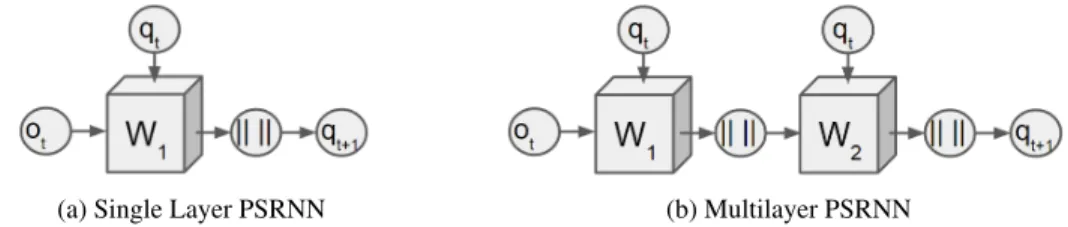
Letqtandotbe the state and observation at timet. LetWbe a 3-mode tensor, and letqbe a vector. The 1-layer state update for a PSRNN is defined as:
qt+1=
W×2ot×3qt+b
kW×2ot×3qt+bk2
(5)
Here the 3-mode tensor of weightsWand the bias vectorbare the model parameters. This architecture is illustrated in Figure 1a. It is similar, but not identical, to the PSR update (Eq. 1); sec 3.1 gives
2
more detail on the relationship. This model may appear simple, but crucially the tensor contraction W×2ot×3qtintegrates information frombtandotmultiplicatively, and acts as a gating mechanism, as discussed in more detail in section 5.
The typical approach used to increase modeling capability for BFs (including PSRs) is to use an initial fixed nonlinearity to map inputs up into a higher-dimensional space [31, 30]. PSRNNs incorporate such a step, via RFFs. However, a multilayered architecture typically offers higher representation power for a given number of parameters [32].
To obtain a multilayer PSRNN, we stack the 1-layer blocks of Eq. (5) by providing the output of one layer as the observation for the next layer. (The state input for each layer remains the same.) In this way we can obtain arbitrarily deep RNNs. This architecture is displayed in Figure 1b.
We choose to chain on the observation (as opposed to on the state) as this architecture leads to a natural extension of 2SR to multilayered models (see Sec. 4.2). In addition, this architecture is consistent with the typical approach for constructing multilayered LSTMs/GRUs [12]. Finally, this architecture is suggested by the full normalized form of an HSE PSR, where the observation is passed through two layers.
(a) Single Layer PSRNN (b) Multilayer PSRNN
Figure 1: PSRNN architecture: See equation 5 for details. We omit bias terms to avoid clutter.
4.2 Learning PSRNNs
There are two components to learning PSRNNs: an initialization procedure followed by gradient-based refinement. We first show how a statistically consistent 2SR algorithm derived for PSRs can be used to initialize the PSRNN model; this model can then be refined via BPTT. We omit the BPTT equations as they are similar to existing literature, and can be easily obtained via automatic differentiation in a neural network library such as PyTorch or TensorFlow.
The Kernel Bayes Rule portion of the PSR update (equation 1) can be separated into two terms:
(W ×3qt)and(Z×3qt)−1. The first term corresponds to calculating the joint distribution, while the second term corresponds to normalizing the joint to obtain the conditional distribution. In the discrete case, this is equivalent to dividing the joint distribution offt+1andotby the marginal ofot; see [33] for details.
If we remove the normalization term, and replace it with two-norm normalization, the PSR update becomesqt+1= kW×W×33qqt×2ot
t×2otk, which corresponds to calculating the joint distribution (up to a scale factor), and has the same functional form as our single-layer PSRNN update equation (up to bias).
It is not immediately clear that this modification is reasonable. We show in appendix B that our algorithm is consistent in the discrete (realizable) setting; however, to our current knowledge we lose the consistency guarantees of the 2SR algorithm in the full continuous setting. Despite this we determined experimentally that replacing full normalization with two-norm normalization appears to have a minimal effect on model performance prior to refinement, and results in improved performance after refinement. Finally, we note that working with the (normalized) joint distribution in place of the conditional distribution is a commonly made simplification in the systems literature, and has been shown to work well in practice [34].
statesqˆ1, ...,qnˆ in place of observations. This process can be repeated as many times as desired to initialize an arbitrarily deep PSRNN. If the first layer were learned perfectly, the second layer would be superfluous; however, in practice, we observe that the second layer is able to learn to improve on the first layer’s performance.
Once we have obtained a PSRNN using the 2SR approach described above, we can use BPTT to refine the PSRNN. We note that we choose to use 2-norm divisive normalization because it is not practical to perform BPTT through the matrix inverse required in PSRs: the inverse operation is ill-conditioned in the neighborhood of any singular matrix. We observe that 2SR provides us with an initialization which converges to a good local optimum.
4.3 Factorized PSRNNs
In this section we show how the PSRNN model can be factorized to reduce the number of parameters prior to applying BPTT.
Let(W, b0)be a PSRNN block. Suppose we decomposeW using CP decomposition to obtain
W =
n
X
i=1
ai⊗bi⊗ci
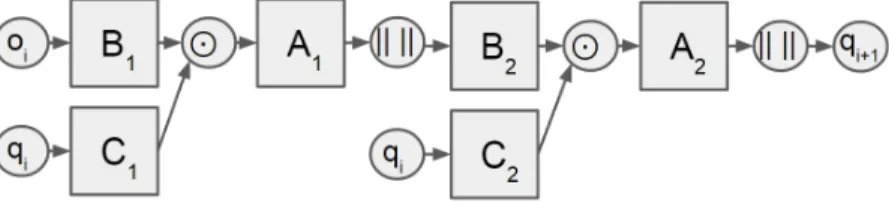
LetA(similarlyB,C) be the matrix whoseith row isai(respectivelybi,ci). Then the PSRNN state update (equation (5)) becomes (up to normalization):
qt+1=W ×2ot×3qt+b (6)
= (A⊗B⊗C)×2ot×3qt+b (7)
=AT(Bot⊙Cqt) +b (8)
where ⊙ is the Hadamard product. We call a PSRNN of this form afactorized PSRNN. This model architecture is illustrated in Figure 2. Using a factorized PSRNN provides us with complete control over the size of our model via the rank of the factorization. Importantly, it decouples the number of model parameters from the number of states, allowing us to set these two hyperparameters independently.
Figure 2: Factorized PSRNN Architecture
We determined experimentally that factorized PSRNNs are poorly conditioned when compared with PSRNNs, due to very large and very small numbers often occurring in the CP decomposition. To alleviate this issue, we need to initialize the biasbin a factorized PSRNN to be a small multiple of the mean state. This acts to stabilize the model, regularizing gradients and preventing us from moving away from the good local optimum provided by 2SR.
We note that a similar stabilization happens automatically in randomly initialized RNNs: after the first few iterations the gradient updates cause the biases to become non-zero, stabilizing the model and resulting in subsequent gradient descent updates being reasonable. Initialization of the biases is only a concern for us because we do not want the original model to move away from our carefully prepared initialization due to extreme gradients during the first few steps of gradient descent.
5
Discussion
The value of bilinear units in RNNs was the focus of recent work by Wu et al [35]. They introduced the concept of Multiplicative Integration (MI) units — components of the formAx⊙By— and showed that replacing additive units by multiplicative ones in a range of architectures leads to significantly improved performance. As Eq. (8) shows, factorizingWleads precisely to an architecture with MI units.
Modern RNN architectures such as LSTMs and GRUs are known to outperform traditional RNN architectures on many problems [12]. While the success of these methods is not fully understood, much of it is attributed to the fact that these architectures possess a gating mechanism which allows them both to remember information for a long time, and also to forget it quickly. Crucially, we note that PSRNNs also allow for a gating mechanism. To see this consider a single entry in the factorized PSRNN update (omitting normalization).
[qt+1]i=
X
j
Aji X k
Bjk[ot]k⊙
X
l
Cjl[qt]l
!
+b (9)
The current stateqtwill only contribute to the new state if the functionP
kBjk[ot]kofotis non-zero. Otherwiseotwill cause the model to forget this information: the bilinear component of the PSRNN architecture naturally achieves gating.
We note that similar bilinear forms occur as components of many successful models. For example, consider the (one layer) GRU update equation:
zt=σ(Wzot+Uzqt+cz)
rt=σ(Wrot+Urqt+cr)
qt+1=zt⊙qt+ (1−zt)⊙σ(Whot+Uh(rt⊙qt) +ch)
The GRU update is a convex combination of the existing stateqtand and update termWhot+Uh(rt⊙
qt) +ch. We see that the core part of this update termUh(rt⊙qt) +chbears a striking similarity to our factorized PSRNN update. The PSRNN update is simpler, though, since it omits the nonlinearity σ(·), and hence is able to combine pairs of linear updates inside and outsideσ(·)into a single matrix. Finally, we would like to highlight the fact that, as discussed in section 5, the bilinear form shared in some form by these models (including PSRNNs) resembles the first component of the Kernel Bayes Rule update function. This observation suggests that bilinear components are a natural structure to use when constructing RNNs, and may help explain the success of the above methods over alternative approaches. This hypothesis is supported by the fact that there are no activation functions (other than divisive normalization) present in our PSRNN architecture, yet it still manages to achieve strong performance.
6
Experimental Setup
In this section we describe the datasets, models, model initializations, model hyperparameters, and evaluation metrics used in our experiments.
We use the following datasets in our experiments:
• Penn Tree Bank (PTB)This is a standard benchmark in the NLP community [36]. Due to hardware limitations we use a train/test split of 120780/124774 characters.
• Swimmer We consider the 3-link simulated swimmer robot from the open-source package OpenAI gym.3 The observation model returns the angular position of the nose as well as the
angles of the two joints. We collect 25 trajectories from a robot that is trained to swim forward (via the cross entropy with a linear policy), with a train/test split of 20/5.
• MocapThis is a Human Motion Capture dataset consisting of 48 skeletal tracks from three human subjects collected while they were walking. The tracks have 300 timesteps each, and are from a Vicon motion capture system. We use a train/test split of 40/8. Features consist of the 3D positions of the skeletal parts (e.g., upper back, thorax, clavicle).
3
• HandwritingThis is a digit database available on the UCI repository [37, 38] created using a pressure sensitive tablet and a cordless stylus. Features arexandytablet coordinates and pressure levels of the pen at a sampling rate of 100 milliseconds. We use 25 trajectories with a train/test split of 20/5.
Models compared are LSTMs [30], GRUs [13], basic RNNs [14], KFs [3], PSRNNs, and factorized PSRNNs. All models except KFs consist of a linear encoder, a recurrent module, and a linear decoder. The encoder maps observations to a compressed representation; in the context of text data it can be viewed as a word embedding. The recurrent module maps a state and an observation to a new state and an output. The decoder maps an output to a predicted observation.4 We initialize the LSTMs and
RNNs with random weights and zero biases according to the Xavier initialization scheme [39]. We initialize the the KF using the 2SR algorithm described in [7]. We initialize PSRNNs and factorized PSRNNs as described in section 3.1.
In two-stage regression we use a ridge parameter of10(−2)nwherenis the number of training examples (this is consistent with the values suggested in [8]). (Experiments show that our approach works well for a wide variety of hyperparameter values.) We use a horizon of 1 in the PTB experiments, and a horizon of 10 in all continuous experiments. We use 2000 RFFs from a Gaussian kernel, selected according to the method of [28], and with the kernel width selected as the median pairwise distance. We use 20 hidden states, and a fixed learning rate of1in all experiments. We use a BPTT horizon of 35 in the PTB experiments, and an infinite BPTT horizon in all other experiments. All models are single layer unless stated otherwise.
We optimize models on the PTB using Bits Per Character (BPC) and evaluate them using both BPC and one-step prediction accuracy (OSPA). We optimize and evaluate all continuous experiments using the Mean Squared Error (MSE).
7
Results
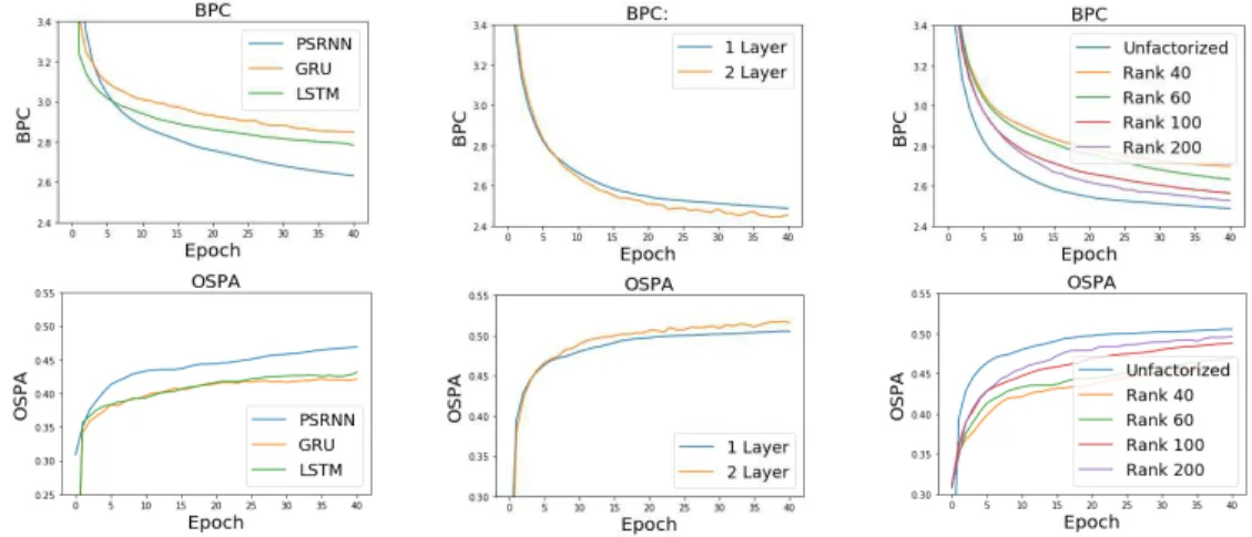
In Figure 3a we compare performance of LSTMs, GRUs, and Factorized PSRNNs on PTB, where all models have the same number of states and approximately the same number of parameters. To achieve this we use a factorized PSRNN of rank 60. We see that the factorized PSRNN significantly outperforms LSTMs and GRUs on both metrics. In Figure 3b we compare the performance of 1- and 2-layer PSRNNs on PTB. We see that adding an additional layer significantly improves performance.
4This is a standard RNN architecture; e.g., a PyTorch implementation of this architecture for text prediction
can be found athttps://github.com/pytorch/examples/tree/master/word_language_model.
(a) BPC and OSPA on PTB. All models have the same number of states and approximately the same number of parameters.
(b) Comparison between 1- and 2-layer PSRNNs on PTB.
(c) Cross-entropy and prediction accuracy on Penn Tree Bank for PSRNNs and factorized PSRNNs of various rank.
In Figure 3c we compare PSRNNs with factorized PSRNNs on the PTB. We see that PSRNNs outperform factorized PSRNNs regardless of rank, even when the factorized PSRNN has significantly more model parameters. (In this experiment, factorized PSRNNs of rank 7 or greater have more model parameters than a plain PSRNN.) This observation makes sense, as the PSRNN provides a simpler optimization surface: the tensor multiplication in each layer of a PSRNN is linear with respect to the model parameters, while the tensor multiplication in each layer of a Factorized PSRNN is bilinear. In addition, we see that higher-rank factorized models outperform lower-rank ones. However, it is worth noting that even models with low rank still perform well, as demonstrated by our rank 40 model still outperforming GRUs and LSTMs, despite having fewer parameters.
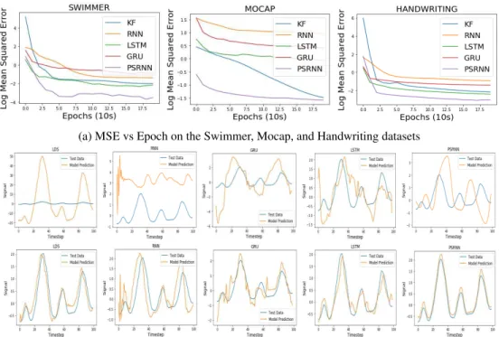
(a) MSE vs Epoch on the Swimmer, Mocap, and Handwriting datasets
(b) Test Data vs Model Prediction on a single feature of Swimmer. The first row shows initial performance. The second row shows performance after training. In order the columns show KF, RNN, GRU, LSTM, and PSRNN.
Figure 4: Swimmer, Mocap, and Handwriting Experiments
In Figure 4a we compare model performance on the Swimmer, Mocap, and Handwriting datasets. We see that PSRNNs significantly outperform alternative approaches on all datasets. In Figure 4b we attempt to gain insight into why using 2SR to initialize our models is so beneficial. We visualize the the one step model predictions before and after BPTT. We see that the behavior of the initialization has a large impact on the behavior of the refined model. For example the initial (incorrect) oscillatory behavior of the RNN in the second column is preserved even after gradient descent.
8
Conclusions
We present PSRNNs: a new approach for modelling time-series data that hybridizes Bayes filters with RNNs. PSRNNs have both a principled initialization procedure and a rich functional form. The basic PSRNN block consists of a 3-mode tensor, corresponding to bilinear combination of the state and observation, followed by divisive normalization. These blocks can be arranged in layers to increase the expressive power of the model. We showed that tensor CP decomposition can be used to obtain factorized PSRNNs, which allow flexibly selecting the number of states and model parameters. We showed how factorized PSRNNs can be viewed as both an instance of Kernel Bayes Rule and a gated architecture, and discussed links to existing multiplicative architectures such as LSTMs. We applied PSRNNs to 4 datasets and showed that we outperform alternative approaches in all cases.
References
[1] Sam Roweis and Zoubin Ghahramani. A unifying review of linear gaussian models. Neural Comput., 11(2):305–345, February 1999. ISSN 0899-7667. doi: 10.1162/089976699300016674. URLhttp://dx.doi.org/10.1162/089976699300016674.
[2] Leonard E. Baum and Ted Petrie. Statistical inference for probabilistic functions of finite state markov chains. The Annals of Mathematical Statistics, 37:1554–1563, 1966.
[3] R. E. Kalman. A new approach to linear filtering and prediction problems. ASME Journal of Basic Engineering, 1960.
[4] Michael L. Littman, Richard S. Sutton, and Satinder Singh. Predictive representations of state. InIn Advances In Neural Information Processing Systems 14, pages 1555–1561. MIT Press, 2001.
[5] Byron Boots, Sajid Siddiqi, and Geoffrey Gordon. Closing the learning planning loop with predictive state representations.International Journal of Robotics Research (IJRR), 30:954–956, 2011.
[6] Byron Boots and Geoffrey Gordon. An online spectral learning algorithm for partially observable nonlinear dynamical systems. InProceedings of the 25th National Conference on Artificial Intelligence (AAAI), 2011.
[7] Ahmed Hefny, Carlton Downey, and Geoffrey J. Gordon. Supervised learning for dynamical system learning. InAdvances in Neural Information Processing Systems, pages 1963–1971, 2015.
[8] Byron Boots, Geoffrey J. Gordon, and Arthur Gretton. Hilbert space embeddings of predictive state representations. CoRR, abs/1309.6819, 2013. URL http://arxiv.org/abs/1309. 6819.
[9] Daniel J. Hsu, Sham M. Kakade, and Tong Zhang. A spectral algorithm for learning hidden markov models. CoRR, abs/0811.4413, 2008.
[10] Amirreza Shaban, Mehrdad Farajtabar, Bo Xie, Le Song, and Byron Boots. Learning latent variable models by improving spectral solutions with exterior point methods. InProceedings of The International Conference on Uncertainty in Artificial Intelligence (UAI), 2015.
[11] Peter Van Overschee and Bart De Moor. N4sid: numerical algorithms for state space subspace system identification. In Proc. of the World Congress of the International Federation of Automatic Control, IFAC, volume 7, pages 361–364, 1993.
[12] Sepp Hochreiter and Jürgen Schmidhuber. Long short-term memory. Neural Comput., 9(8): 1735–1780, November 1997. ISSN 0899-7667. doi: 10.1162/neco.1997.9.8.1735.
[13] KyungHyun Cho, Bart van Merrienboer, Dzmitry Bahdanau, and Yoshua Bengio. On the properties of neural machine translation: Encoder-decoder approaches.CoRR, abs/1409.1259, 2014.
[14] Jeffrey L. Elman. Finding structure in time.COGNITIVE SCIENCE, 14(2):179–211, 1990.
[15] Ilya Sutskever, Oriol Vinyals, and Quoc V. Le. Sequence to sequence learning with neural networks. CoRR, abs/1409.3215, 2014. URLhttp://arxiv.org/abs/1409.3215.
[16] Byron Boots. Learning stable linear dynamical systems.Online]. Avail.: https://www. ml. cmu. edu/research/dap-papers/dap_boots. pdf, 2009.
[17] Yuchen Zhang, Xi Chen, Denny Zhou, and Michael I Jordan. Spectral methods meet em: A provably optimal algorithm for crowdsourcing. InAdvances in neural information processing systems, pages 1260–1268, 2014.
[19] Peter Van Overschee and Bart De Moor. N4sid: Subspace algorithms for the identification of combined deterministic-stochastic systems. Automatica, 30(1):75–93, January 1994. ISSN 0005-1098. doi: 10.1016/0005-1098(94)90230-5. URL http://dx.doi.org/10.1016/ 0005-1098(94)90230-5.
[20] Luca Pasa, Alberto Testolin, and Alessandro Sperduti. A hmm-based pre-training approach for sequential data. In 22th European Symposium on Artificial Neural Networks, ESANN 2014, Bruges, Belgium, April 23-25, 2014, 2014. URL http://www.elen.ucl.ac.be/ Proceedings/esann/esannpdf/es2014-166.pdf.
[21] David Belanger and Sham Kakade. A linear dynamical system model for text. In Francis Bach and David Blei, editors,Proceedings of the 32nd International Conference on Machine Learning, volume 37 ofProceedings of Machine Learning Research, pages 833–842, Lille, France, 07–09 Jul 2015. PMLR.
[22] James Martens. Learning the linear dynamical system with asos. InProceedings of the 27th International Conference on Machine Learning (ICML-10), pages 743–750, 2010.
[23] Carlton Downey, Ahmed Hefny, and Geoffrey Gordon. Practical learning of predictive state representations. Technical report, Carnegie Mellon University, 2017.
[24] Tuomas Haarnoja, Anurag Ajay, Sergey Levine, and Pieter Abbeel. Backprop kf: Learning discriminative deterministic state estimators. InAdvances in Neural Information Processing Systems, pages 4376–4384, 2016.
[25] Jean Kossaifi, Zachary C Lipton, Aran Khanna, Tommaso Furlanello, and Anima Anandkumar. Tensor regression networks. arXiv preprint arXiv:1707.08308, 2017.
[26] Alex Smola, Arthur Gretton, Le Song, and Bernhard Schölkopf. A hilbert space embedding for distributions. InInternational Conference on Algorithmic Learning Theory, pages 13–31. Springer, 2007.
[27] Nachman Aronszajn. Theory of reproducing kernels.Transactions of the American mathemati-cal society, 68(3):337–404, 1950.
[28] Ali Rahimi and Benjamin Recht. Random features for large-scale kernel machines. InAdvances in neural information processing systems, pages 1177–1184, 2008.
[29] Frank L Hitchcock. The expression of a tensor or a polyadic as a sum of products. Studies in Applied Mathematics, 6(1-4):164–189, 1927.
[30] Lennart Ljung.System identification. Wiley Online Library, 1999.
[31] Le Song, Byron Boots, Sajid M. Siddiqi, Geoffrey J. Gordon, and Alex J. Smola. Hilbert space embeddings of hidden markov models. In Johannes Fürnkranz and Thorsten Joachims, editors,
Proceedings of the 27th International Conference on Machine Learning (ICML-10), pages 991–998. Omnipress, 2010. URLhttp://www.icml2010.org/papers/495.pdf.
[32] Yoshua Bengio et al. Learning deep architectures for ai.Foundations and trendsR in Machine Learning, 2(1):1–127, 2009.
[33] Le Song, Jonathan Huang, Alex Smola, and Kenji Fukumizu. Hilbert space embeddings of conditional distributions with applications to dynamical systems. InProceedings of the 26th Annual International Conference on Machine Learning, pages 961–968. ACM, 2009.
[34] Sebastian Thrun, Wolfram Burgard, and Dieter Fox. Probabilistic robotics. MIT press, 2005.
[35] Yuhuai Wu, Saizheng Zhang, Ying Zhang, Yoshua Bengio, and Ruslan Salakhutdinov. On multiplicative integration with recurrent neural networks. CoRR, abs/1606.06630, 2016. URL http://arxiv.org/abs/1606.06630.
[37] Fevzi. Alimoglu E. Alpaydin. Pen-Based Recognition of Handwritten Digits Data Set. https://archive.ics.uci.edu/ml/datasets/Pen-Based+Recognition+of+Handwritten+Digits.
[38] E Alpaydin and Fevzi Alimoglu. Pen-based recognition of handwritten digits data set.University of California, Irvine, Machine Learning Repository. Irvine: University of California, 1998.