The accessibility to the nearest urban
metropolitan area and rural poverty in Japan
journal or
publication title
DSSR Discussion Papers
number
86
page range
1-19
year
2018-05
URL
http://hdl.handle.net/10097/00122650
Data Science and Service Research
Discussion Paper
Discussion Paper No. 86
The accessibility to the nearest urban
metropolitan area and rural poverty in Japan
Takeru Sugasawa
May, 2018
Center for Data Science and Service Research
Graduate School of Economic and Management
Tohoku University
27-1 Kawauchi, Aobaku
Sendai 980-8576, JAPAN
The accessibility to the nearest urban metropolitan area and rural poverty in Japan
Takeru Sugasawa†Abstract
This study examines the effects of accessibility to the nearest urban metropolitan area on rural poverty by using Japanese municipality-level data. We conduct nationwide cross-sectional analyses and Ibaraki prefecture’s, a suburban area of Tokyo, municipality-level panel analyses. we find that a larger time distance to the nearest urban metropolitan area significantly increases regional poverty rates. The results of the panel analyses suggest that the effects of reducing rural poverty require 6–10 years to be observed. Therefore, regional policy makers might need to consider that transportation investments that improve inter-regional accessibility do not affect regional economic performance for several years.
JEL classification:R11 R12 R13R41R42
1. Introduction
Even in developed countries, poverty is still a serious problem, and improving income levels is crucial for reducing poverty ILO (2016). As empirical evidence of the relationship between income level and poverty,Förster and Mira (2005) examine the case of OECD countries in the second half of the 1990s and find that their poverty rates and income levels strongly correlate. From those discussions, there is a possibility that factors affecting regional income levels also have impacts on regional poverty situations.
As an important factor that affects regional economic performance, we consider agglomeration spillover effects. Marshall (1920) mentions the possibility that firms tend to concentrate to get advantages such as rich labor markets, low transportation costs of inputs and outputs, and knowledge spillover. Moreover, Rosenthal and Strange (2004) point out that firms receive the benefits of home market effects, opportunity of urban consumption, and rent seeking in addition to the agglomeration advantages
suggested by Marshall. Those benefits of agglomeration increase the productivity of firms in urban metropolitan areas, and the effects are known to spill over to surrounding regions.
The magnitude of agglomeration spillover effects is known to diminish by distance from urban metropolitan areas. Jaffe et al. (1993) investigate the location of patent citations in the United States and find that domestic patents tend to be cited in the states and standard metropolitan statistical areas of the
† the Department of Economics and Management, Tohoku University (tel: 090-8478-3247, e-mail: [email protected])
patents. They also suggest that the diffusing of domestic patents to surrounding areas occurs very slowly. Moreover, Adams and Jaffe (1996) focus on the relationship between plant-level productivity and firm-level research and development activities (R&D) and find that the positive effects of firms’ R&D on plants’ productivity diminish with the distance between the plants and the research labs. The above discussions suggest that positive agglomeration spillover effects are attenuated by distance, and there is a possibility that a larger distance from closely located urban metropolitan areas causes a lower regional wage level and worsens regional poverty situations.
In this study, we estimate the effects of accessibility to the nearest urban metropolitan area on regional poverty by using Japanese municipality-level data. From our nationwide cross-sectional
analyses, we find that a larger time distance to the nearest urban metropolitan area significantly increases regional poverty rates. The monetary magnitude is such that a one-minute increase of time distance to the nearest urban metropolitan area increases the number of households in poverty by about 0.78, and it increases the annual expenditure of regional governments for public assistance by about 1.75 million yen on average in 2014.
In addition, we focus on the case of a new commuting train that opened in 2005, the Tsukuba Express (TX), which connects Tokyo and suburban areas, and conduct panel analyses to understand the impacts of changing accessibility to closely located urban metropolitan areas on rural poverty. From our panel analysis, we find that improvements in accessibility to the nearest urban metropolitan area significantly decreases poverty rates, even controlling for municipality fixed effects. We also find that the effects of reducing regional poverty are observed in municipalities located close to TX. The result is consistent with our hypothesis that improvement in accessibility to the nearest urban metropolitan area will spread the range of positive spillover effects from urban metropolitan areas, stimulate their economic performance, and reduce poverty.
In a related study, Partridge and Rickman (2008) investigate the relationship between regional poverty rates and distance from the nearest urban metropolitan areas by using county-level data from the United States, showing that larger linear distance from a nearby urban metropolitan areas causes higher poverty rates in counties. However, there are two issues that are not considered in their study. First, Partridge and Rickman use linear distance as a distance variable, which cannot measure accurate inter-regional accessibility1. To solve the problem, we adopt time distance, which can measure actual transportation
1 Boscoe, Henry, and Zdeb (2012) focus on the relationship between housing prices and distance to the nearest hospital in the case of the United States, the District of Colombia and Puerto Rico. They find that linear distance does not work appropriately as a measure of accessibility if there are geographic barriers that prevent people from travaling.
costs as an inter-regional accessibility variable, as well as linear distance. From our estimations, a larger time distance to the nearest urban metropolitan area causes higher regional poverty rates, while linear distance to the nearest urban metropolitan area does not explain rural poverty. Second, Partridge and Rickman (2008) only conduct a cross-sectional analysis, and their results may contain biases from neglecting unobservable regional characteristics. Against this background, we conduct a panel analysis to understand the effects of changing transportation costs to closely located urban metropolitan areas on rural poverty rates, controlling for time invariant regional characteristics, and find that the opening of a new commuting train reduces poverty in regions located close to the commuting train.
The structure of this paper is as follows. The next section describes the mechanism of the relationship whereby access to urban metropolitan areas affects rural poverty, in reference to previous studies. Section 3 explains our estimation models and variables. Section 4 describes the results of the cross-sectional analysis. Section 5 describes the configuration of the panel analysis and its results. Section 6 is the conclusion.
2. Background mechanism
This section describes the mechanism whereby regional accessibility to closely located urban metropolitan areas affects rural poverty, referring to previous studies. The seriousness of the poverty situation in a region depends on the regional wage and employee level, which is determined as an equilibrium of regional labor demand and labor supply. Partridge and Rickman (2008) formulate the relationship whereby regional employment and wage rates affect regional poverty, which can be written as the following function.
Poverty(= f(,-./𝑒𝑟(, 𝑤𝑟(, 𝒐𝒕𝒉𝒆𝒓𝒊𝒑𝒐𝒗<, (1) where 𝑒𝑟( is the employment rate of region i and 𝑤𝑟( is its wage rate. 𝒐𝒕𝒉𝒆𝒓𝒊
𝒑𝒐𝒗
is the vector of other variables that affect the poverty situation of region i. To understand how Poverty( exerts influence, we consider how 𝑒𝑟( and 𝑤𝑟( exert influence.
The employee and wage rates of a region depend on the interaction between regional labor demand and labor supply. The relationships are written as the following functions.
𝑒𝑟(= f@AB /𝑙 (D, 𝑙 (E<, (2) 𝑤𝑟(= f@GB/𝑙 (D, 𝑙 (E<, (3)
where 𝑙 (D is the labor demand of region i, and 𝑙 (E is the labor supply. If other factors are given, an increase of 𝑙 (D increases 𝑒𝑟( or 𝑤𝑟(, and an increase of 𝑙 (E decreases 𝑒𝑟( or 𝑤𝑟(. Then, we consider factors that determine the level of regional labor demand and labor supply.
On the labor demand side, agglomeration economy spillovers and increases in the labor demand of the surrounding regions occur, and the spillover effects are known to diminish by distance. Rosenthal and Strange (2003 and 2006) focus on six kinds of industries’ agglomeration and the ranges of their spillover effects in the United States. Their results suggest that the amount of employment rapidly diminishes by distance from agglomeration in five out of six industries. In addition, Audretsch et al. (2005) focus on knowledge spillover effects from universities on new establishments of high technology-based firms in the United States. They find that high technology-based firms tend to locate close to universities, and those firms are strongly concentrated within 50 kilometers of universities. The above studies suggest that the amount of regional labor demand decreases by distance from economic agglomeration.
On the labor supply side, rural workers are known to have difficultly accessing urban labor markets across regions. Lucas (2001) introduces evidence suggesting that rural workers stay in their own areas in spite of higher income levels in urban metropolitan areas. Molho (1995) provides one of the evidences referenced in Lucas (2001), suggesting that rural workers tend to stay in rural areas because of their attachment to the culture or human relations in areas in which they live. In addition, Lucas (2001) identifies information costs about urban labor markets, which become larger by distance from urban metropolitan areas, as a reason that rural workers stay in the areas in which they live.
The above discussions suggest that whereas labor demand concentrates in urban metropolitan areas and the amount rapidly diminishes by distance from economic agglomeration, rural workers’ mobility is at a low level and they have difficulty migrating to urban metropolitan areas across regions in pursuit of higher wages. This causes the amount of labor demand to diminish by distance from economic
agglomeration with a larger slope than that of the labor supply. We can express the relationships as the following functions: 𝑙 (D= fIJ/𝐷𝑖𝑠𝑡𝑎𝑛𝑐𝑒(RS, 𝒐𝒕𝒉𝒆𝒓𝒊𝒍𝒅<, VW XY VZ(E[\]^_X`a< 0, (4) 𝑙 (E = fId/𝐷𝑖𝑠𝑡𝑎𝑛𝑐𝑒(RS, 𝒐𝒕𝒉𝒆𝒓𝒊𝒍𝒔<, VW Xf gZ(E[\]^_X`a< 0, (5) VW XY VZ(E[\]^_X`a < VW Xf gZ(E[\]^_X`a, (6) where 𝐷𝑖𝑠𝑡𝑎𝑛𝑐𝑒(RS is the distance to the nearest urban metropolitan area of region i. From functions (2) and (3), increases of 𝐷𝑖𝑠𝑡𝑎𝑛𝑐𝑒(RS decrease regional wages or employees level through changes of 𝑙 (D
and 𝑙 (E, and from function (1), the increases of 𝐷𝑖𝑠𝑡𝑎𝑛𝑐𝑒(RS cause a worsening of the regional poverty situation. The relationship can be written as the following function:
poverty(= f@
ijk(𝐷𝑖𝑠𝑡𝑎𝑛𝑐𝑒
(RS, 𝒐𝒕𝒉𝒆𝒓𝒊),
VijkABlmn
VZ(E[\]^_X`a> 0, (7)
where poverty( is the poverty rate of region i.
From the above discussion, we assume that better accessibility to closely located economic
agglomeration improve the regional poverty situation. We examine the impact of distance to the nearest urban metropolitan area on rural poverty rates with Japanese municipality level data.
3. Cross-sectional analysis 3.1. Empirical strategy
Based on the theoretical background, this section describes the estimation model that explains the level of municipalities’ poverty rates. The estimation model is as follows:
Pov(= 𝛼(+ βDistance(+ δ𝐗𝒊+ θPrefecture( + u(. (8)
Pov( is municipality i’s poverty rate. Distance( is municipality i’s distance to the nearest urban metropolitan area. According to the above discussion, we expect that β is negative.
𝐗𝒊 is the vector that contains variables relating to municipality i’s poverty rate. It contains three types of variables, explaining municipality i’s population structure, economic activity, and education level. Prefecture( is a prefecture dummy in which municipality i is contained. We adopt it to control for the heterogeneity that comes from the prefecture of municipality i. u( is the error term.
3.2. Data
This section describes the data we use. First, we clarify the definition of municipalities and urban metropolitan areas.
The Japanese government defines a municipality as the smallest unit of administrative districts, and it is composed of cities, towns, villages, and specified districts2. We define urban metropolitan areas as municipalities with populations of over 300,000; that is a condition of the core city, which is a legal urban metropolitan area determined by article 252 of the Local Autonomy Law3. In Japan, there were 71 urban
2 In 2012, there were 1747 municipalities composed of 786 cities, 754 towns, 184 villages and 23 specified districts in the Tokyo metropolitan area.
3 In 2016, the definition of core city changed to cities with a population over 200,000. However, we adopt the previous definition used in 2012, in which our sample is observed.
metropolitan areas in 2012. In addition, we regard 23 specified districts in the Tokyo metropolitan area as one urban metropolitan area. In this study, each municipality has a nearest urban metropolitan area. The nearest urban metropolitan area of a municipality is defined as the urban metropolitan area that has the closest linear distance to the rural municipality.
To conduct cross-sectional analysis, we except municipalities that are urban metropolitan areas themselves and use only rural municipalities with populations under 300,000 as our sample. The reason for this is that we cannot observe the distribution of poverty in each municipality and cannot calculate the distance between poor households in urban areas and the nearest urban metropolitan area. That renders us unable to estimate the effects of distance to the urban metropolitan area located in the municipality on regional poverty rates.
Distance( is municipality i’s distance to the nearest urban metropolitan area. In our cross-sectional analysis, we adopt linear distance, time distance by car, and time distance by public transport as accessibility variables to the nearest urban metropolitan area.
Linear distance is measured as the linear distance by kilometer between the government offices of a rural municipality and the municipality’s nearest urban metropolitan area. We calculate the linear distance between municipalities using a location-based service and coordinate conversion service from the
Geospatial Information Authority of Japan.
Time distance by car measures how long people would spend to travel between two government offices by car. This variable is calculated using Google Maps. Time distance by public transport is the time people spend to travel between the municipality in which they live and its nearest urban metropolitan area by train and bus4. We calculate this variable using the Timetable published by the Japan Travel Bureau (JTB), which is a representative time table of public transportation in Japan. In the case of municipalities that contain stations, we measure the time distance between their representative station, which is defined in the Timetables, and the representative station of its nearest urban metropolitan area. In the case of municipalities that do not contain stations in them, we add the time distance between their governments office’s nearest bus stop and its nearest station to the time distance from the rural station to the representative station of its nearest urban metropolitan area. We calculate the optimal path between a rural municipality and its nearest urban metropolitan area for commuters5. The unit of time distance is one minute.
4 A municipality’s principal station is defined by each government of the municipality.
5 The optimal path is calculated as the fastest path from a rural station to the representative station of the nearest urban metropolitan area, but we except limited express trains and bullet trains, which require additional fare as commuting methods.
As the measure of regional poverty rates, we adopt a municipality’s share of households receiving public assistance. This is defined as the ratio of households receiving public assistance to 100 households in each municipality. The requirement for receiving public assistance is that a household lives under the poverty line, which is determined by the standards created by the Ministry of Health, Labour and Welfare (MHLW). Each municipality’s income threshold for providing public assistance controls for each municipality’s price level determined by MHLW. We assume that municipalities’ share of households receiving public assistance work as a proxy for the absolute poverty rate, which is defined as “the
inability to meet basic needs of health and nutrition” Deaton (2004). To calculate the public assistance
rate of each municipality, we use the Prefectural Statistic Manuals (2012).
Partridge and Rickman (2008) use the poverty standard that is defined by the U.S. Census Bureau. The standard aims to identify whether a household is in an absolute poverty situation, and it controls for states’ price levels and the number of household members; it has similar requirements to those of the Japanese income threshold for receiving public assistance. The similarity between the two poverty standards is convenient for us to compare our estimation results with those of Partridge and Rickman (2008).
Using 𝐗𝒊, we control for factors relating to municipality i’s poverty rate. It contains three types of variables. (I) The variables that explain municipality i’s population structure are the number of
households and age structure (the share of population under 15 and the share of population over 65). (Ⅱ) The variables about municipality i’s economic performance are industrial structure (share of laborers in the primary sector and in the manufacture sector) and municipality i’s unemployment rate. (Ⅲ) The variables reflecting municipalities’ education level are the share of people who graduate from a university and the share of high school graduates. To obtain those variables, we use the Statistical Observations of Prefectures, constructed by the Ministry of Internal Affairs and Communications Statistics Bureau (2010).
We use 33 prefectures from the total of 47, which announce the share of households receiving public assistance at the municipality level6. Table 1 displays the summary statistics.
4. Cross-sectional results
This section describes the results of our cross-sectional estimation. Table 2 shows the estimation results.
Column (1) uses linear distance as Distance(, and its coefficient is positive and insignificant. This result suggests that linear distance to the nearest urban metropolitan area does not have significant effects on rural poverty rates. Column (2) adopts time distance by car as Distance(. The coefficient is positive with a 10% statistical significance. The magnitude is that one-minute increases of time distance by car to the nearest urban metropolitan area increase the rural poverty rates by about 0.003%. Column (3) shows the
6 The 33 available prefectures are Hokkaido, Iwate, Fukushima, Ibaraki, Tochigi, Saitama, Chiba, Tokyo, Kanagawa, Toyama, Fukui, Gifu, Aichi, Shiga, Kyoto, Osaka, Hyogo, Nara, Wakayama, Tottori, Shimane, Hiroshima, Yamaguchi, Kagawa, Kochi, Fukuoka, Saga, Nagasaki, Kumamoto, Oita, Miyazaki, Kagoshima, and Okinawa.
estimation of time distance by public transport, and its coefficient is positive with a five percent statistical significance. This result shows basically the same result as estimation (2). One minute increases of time distance by public transports to the nearest urban metropolitan area increase rural poverty rates by about 0.002%.
Columns (1)-(3) are fundamentally consistent with the results of Partridge and Rickman (2008) in suggesting that a larger distance to the nearest urban metropolitan area will cause a worsening of the rural poverty situation. However, our results also show that there is difference between the significance of linear distance and time distance. From columns (1)-(3), we find that, whereas a municipality’s linear distance to the nearest urban metropolitan area does not have significant effects on rural poverty rates, time distance significantly affects rural poverty rates. These results suggest that, whereas linear distance does not precisely capture inter-regional accessibility in regions, such as Japan, which have many geographical barriers, time distance could measure accessibility.
We consider the monetary impact of distance to the nearest urban metropolitan area on rural
governments. From column (3)’s result, the magnitude of a one-minute increase of time distance is about a 0.002% increase of rural poverty rates. These results show that, for instance, an increase of 10 minutes of time distance to the nearest urban metropolitan area causes municipalities’ annual expenditures for
public assistance to increase by about 17.5 million yen on average7.
There is a possibility that the scale of economic agglomeration affects the magnitude of spillover effects on surrounding regions. In analyses (4)-(9), we divide municipalities by the scale of population of their nearest urban metropolitan area. We define the threshold of municipalities as whether their nearest
7 In 2014, there were about 56.4 million households in Japan, and about 1.6 million households received public assistance; thus, the share of households receiving public assistance was about 2.38%. There were 1718 municipalities in 2014, and each municipality has about 931 households receiving public assistance on average. The total expenditure of the Japanese government for public assistance was about 3843 billion yen, and, dividing the amount of total expenditure by the number of municipalities, a
municipality’s average expenditure for public assistance was about 2.2 billion yen. From the average number of households receiving public assistance and the amount of the expenditure, the average amount of public assistance for each household was about 2.4 million yen. From the results of (2) and (3), an increase of 10 minutes of time distance increases the share of public assistance by about 0.02; thus, it adds about 7.82 households receiving public assistance. In this result, a municipality’s annual expenditure for public assistance increases by about 17.5 million yen on average.
urban metropolitan area has a population over 500,000; this is one of the requirements to be an ordinance designated city, which is a representative system to define metropolises in Japan. Columns (4)-(6) present the results of estimations (using the municipalities) of which nearest urban metropolitan area has a population larger than 500,000. Columns (7)-(9) use the municipalities that only include municipalities with a population smaller than 500,000.
The results of (4)-(6) suggest that distance to the nearest urban metropolitan area does not have significant effects on rural poverty rates in municipalities whose nearest urban metropolitan area has a population larger than 500,000. From columns (7)-(9), we can observe qualitatively similar results to those of columns (1)-(3) in that the coefficient of linear distance is positive and insignificant, and the coefficients of time distance by car and by public transport are positive and statistically significant. Column (7) uses linear distance as Distance(, and its coefficient is positive and insignificant. Column (8) adopts time distance by car as Distance(. The coefficient is positive with 10% statistical significance. The result shows that one-minute increases of Distance( increase the rural poverty rates by about 0.002%. Column (9) provides the estimation with time distance by public transport, and its coefficient is positive with 10% statistical significance. This result suggests that one-minute increases of Distance( cause rural poverty rates to increase by about 0.002%. Columns (4)-(9) show that whereas distance to the smaller urban metropolitan areas impacts rural poverty rates, accessibility to larger urban metropolitan areas does not have significant effects.
We consider the reason that only municipalities closely located to a smaller urban metropolitan area experience significant effects from distance to urban metropolitan areas. From columns (5) and (8), we find that in municipalities close to a larger urban metropolitan area, the magnitude of the coefficient (about 0.002) is larger than that of municipalities close to a smaller urban metropolitan area (about 0.0018). However, the coefficient for municipalities close to a larger urban metropolitan area has a considerably higher standard error (about 0.0012) than that of municipalities close to a smaller urban metropolitan area (about 0.00075), and that causes the insignificance of time distance in column (5). From columns (5), (6), (8), and (9), we can observe that municipalities close to larger urban metropolitan areas consistently have a larger standard error of time distance to the nearest urban metropolitan areas than municipalities close to smaller urban metropolitan areas. This suggests that there are larger heterogeneities among municipalities close to larger urban metropolitan areas than among those close to smaller urban metropolitan areas; for example, only some of the municipalities receive a large benefit from good accessibility to the nearest urban metropolitan area, and the others do not receive it. We consider that the reason for this is that large urban metropolitan areas resorb the economic activities of surrounding regions and generate regions with inactive economies, which is called the urban shadow
effect. From this discussion, there is a possibility that only some of the municipalities located close to large urban metropolitan areas have their economic activity resorbed by the urban metropolitan areas, which causes a larger dispersion among the surrounding municipalities of large urban metropolitan areas than those of smaller urban metropolitan areas.
Although our estimation model includes all the possible variables to control for municipality heterogeneity, there is a possibility that our model still misses unobservable characteristics cannot be controlled by these variables’ and the results may include some biases. To control for unobservable time invariant heterogeneities of municipalities, we conduct a panel analysis and estimate the impact of improving accessibility to the nearest urban metropolitan area on rural poverty rates.
5. Panel analysis
5.1. The opening of the new Tsukuba Express
To control for unobservable and time invariant characteristics of municipalities, we focus on the case of the opening of the new TX in 2005. TX is a commuting train connecting Tsukuba (a suburban city in Ibaraki prefecture) to Akihabara (a terminal station locating in CBD in Tokyo). Opening TX shortened the time distance between Tsukuba and Akihabara from 60 minutes to 40 minutes. The drastic change of accessibility to urban metropolitan areas might affect the geographic ranges of spillover effects from economic agglomeration on the surrounding regions of the railroad. For instance, households’ job selecting behavior or firms’ decision of location could reflect the impacts of changing accessibility in surrounding municipalities of the railway. Since the railway also contains Kashiwa (an urban
metropolitan area in Chiba) as its passing station, the opening of TX might have impacts that come from the change of accessibility to other smaller urban metropolitan areas as well as to Tokyo. Figure 1 shows the routes of TX and the Joban line, which is an existing railway connecting municipalities in Ibaraki to Tokyo. The route of TX is colored red, and the Joban line is colored blue. Each circle represents a station of the railways.
5.2. Panel analysis
We create panel data and estimate the impacts of accessibility to urban metropolitan areas on
municipalities’ poverty rates, controlling for the time invariant characteristics of municipalities. To create the panel data, we use Timetable (JTB: 2000, 2005, 2010, 2015) and calculate the time distance among stations using the appropriate commuting route. The estimation model is as follows:
η( is municipality fixed effects. ε([ is the error term, which comes from the time invariant characteristics of municipality i.
In our panel analysis, only the time distance by public transport is used as distance variables. Linear distance cannot identify changes of inter-regional accessibility. Additionally, we cannot observe previous time distance by car.
Ibaraki prefecture is divided into five regions: Central, South, West, North and Rokko region8. TX terminates at Tsukuba city, in the South region. Figure 2 shows the regions of Ibaraki prefecture and the
8 Each region is composed of municipalities as follows: Central (Mito, Kasama, and Omitama cities, and Ibaraki, Oarai, and Shirosato towns), South (Tsuchiura, Ishioka, Ryugasaki, Toride, Ushiku, Tsukuba, Inashiki, Kasumigaura, and Thukubamirai cities; Miho village; and Ami and Kawachi towns), West (Koga, Yuki, Shimotsuma, Joso, Chikusei, Bando, and Sakuragawa cities, and Yachiyo town), North (Hitachi, Hitachiota, Takahagi, Kitaibaraki, Hitachinaka, Hitachiomiya, and Naka cities; and Tokai village; and Daigo town), and Rokko region (Kashima, Itako, Kamisu, Namekata, and Hokota cities).
route of TX. Since there is a difference in proximity to the new commuting train among the
municipalities, the impact of opening TX might affect only municipalities that have better accessibility to the new railway. To control for the characteristics of proximity to TX, we introduce a cross-term of TimeDistance([ and an indicator that identifies whether a municipality is close to TX. The estimation model is as follows:
Pov([ = α([+ βTimeDistance([ + γTimeDistance([× ClosetoTX( + δ𝐗([+ η(+ ε([. (10)
We define the closer regions to TX as the West, South, and Rokko regions; if a municipality is included in the regions, the indicator becomes one.
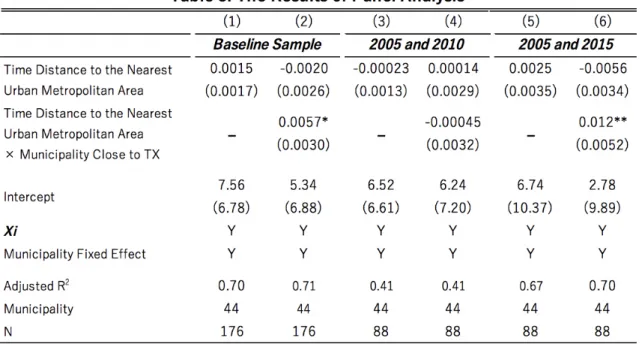
5.3. The results
Table 3 describes the results of our panel analysis. Columns (1)–(2) are the results of the analysis using all of the sample (2000, 2005, 2010, and 2015). In column (1), the coefficient of TimeDistance([ is positive and insignificant. This result shows that time distance to the nearest urban metropolitan area does not affect rural poverty rates. Then we include the interaction term between TimeDistance([ and ClosetoTX( in our model, as well as TimeDistance([. In column (2), the coefficient of TimeDistance([ is negative and insignificant, and the coefficient of the cross term is positive with 10% significance. The magnitude of the interaction term is that one-minute decreases of TimeDistance([ reduce rural poverty rates by about 0.006%.
From columns (1) and (2), we find that accessibility to the nearest urban metropolitan area does not have significant impacts on rural poverty rates overall in the Ibaraki prefecture. However, column (2) suggests that time distance to urban metropolitan areas has impacts on rural poverty in municipalities that are closer to TX. From the results, we find that the opening of TX affected only municipalities that have better accessibility to TX. Although time distance to the nearest urban area also changed in the regions that are not close to TX, their poverty rates did not reflect the changes of accessibility. We consider that a slight change of accessibility to urban metropolitan areas cannot spread or strengthen agglomeration spillover effects enough to cause the rural poverty situation to be improved, but that the opening of the new TX caused a significant improvement of accessibility to urban metropolitan areas, which was enough
to improve the poverty rates of areas peripheral to TX.
Table 4 shows the average time distance to the nearest urban metropolitan area before (2005) and after the (2010) opening of TX. From the table, we find that whereas municipalities close to TX decrease their time distance to the nearest urban metropolitan area by about 8.7 minutes on average, municipalities far from TX decrease their time distance by only about 3.3 minutes. We consider that the difference of magnitude reflects the municipalities’ accessibility to TX, and municipalities close to TX might receive the impact of opening TX more sensitively than municipalities far from TX.
In addition, the difference of impacts of changing accessibility to urban metropolitan areas might be explained by the preference for commuting costs of people in poverty. Roberto (2008) empirically investigates the case of the United States and finds that the working poor have a larger burden of commuting costs than the national median in eight metropolitan cities. The study suggests the possibility that people living in a poor situation have lower price elasticity of commuting costs than people not in poverty. If improved commuting costs to the nearest urban metropolitan area are still too expensive for people in poverty, the municipalities’ poverty situations might not reflect the changing accessibility to urban areas. From this discussion, we consider that a slight change of accessibility to urban areas could not affect rural poverty rates significantly.
There could be some lags between the opening of TX and the economic effects of the new commuting train. Chandra and Thompson (2000) focus on the lag of firms’ relocation after improvements of
suburban regions’ labor demand do not appear significantly until several years later. Their results suggest that improvement of accessibility to a closely located urban metropolitan area will spread ranges of agglomeration spillover effects and increase labor demand in surrounding regions, but some lags occur before the effects appear. Providing that the lags occur in cases of opening commuting trains, there is a possibility that an improvement in poverty rates will not be observed until several years after the TX opening in surrounding areas of TX.
To observe the lags of effects appearing after the TX opening, we conduct panel analyses (3)–(6). Columns (3)–(4) are the results of analyses using periods 2005 and 2010 as the sample. On the other hand, columns (5)–(6) adopt years 2005 and 2015 as the sample. Columns (3) and (5) adopt time distance to the nearest urban metropolitan area as the distance variable. In addition, columns (4) and (6) adopt the cross term between ClosetoTX( and TimeDistance([, as well as TimeDistance([.
In column (3), the coefficient of TimeDistance([ is negative and insignificant. In column (4), the coefficient of TimeDistance([ is positive and insignificant, and one of the cross terms is negative and insignificant. In column (5), the coefficient of TimeDistance([ is positive and insignificant. In column (6), the coefficient of TimeDistance([ is negative and insignificant, and one of the cross terms is positive with five percent statistical significance.
Columns (3)–(4) show that time distance to urban metropolitan areas does not have significant effects on rural poverty rates in 2005 and 2010. However, from columns (5) and (6), we find that one-minute increases of time distance to the nearest urban metropolitan area cause rural poverty rates to increase about 0.012% in municipalities close to TX. The results show that the economic effects of opening TX on the peripheral regions did not appear until 6–10 later. We consider that our results are consistent with the findings of Chandra and Thompson (2000), which suggest that the effects of improvement accessibility to urban metropolitan areas take some years to be observed.
We investigate the relationship between municipalities’ accessibility to the nearest urban metropolitan area and rural poverty rates by focusing on the case of Japanese municipalities. We find that whereas increasing the time distance to the nearest urban metropolitan area increases rural poverty rates, linear distance does not explain the situation of rural poverty. When focusing on the case with many geographical barriers, there will be some difference between linear distance and time distance in explaining the spillover effects of urban agglomeration on regional economic performance.
Moreover, we focus on the impacts of the opening of a commuting train, TX in 2005 on surrounding municipalities’ poverty rates and conduct panel analysis to control for time invariant characteristics of municipalities. Even when we control for regional time invariant characteristics, the causal effects of access to the nearest urban metropolitan area on rural poverty rates are observed significantly in municipalities close to the new commuting train. This result suggests that slight changes of accessibility to the nearest urban metropolitan area do not affect the regional poverty situation significantly.
From our estimations, one-minute increases of time distance to the nearest urban metropolitan area increase rural poverty rates by about 0.002%.This implies that about 0.78 additional households begin to receive public assistance and cause increases of the annual expenditure for public assistance of about 1.75 million yen on average. In addition, we find that the economic effects of opening TX on the surrounding regions did not appear until 6–10 years later. This result suggests that when governments invest in transportation infrastructures to improve their economic performance, they ought to expect that the effects will not appear until a few years later.
Our results show that economic agglomeration spillovers are effective in reducing the poverty of surrounding regions, and improving accessibility to closely located urban metropolitan areas enlarges the magnitude and ranges of the effects. Transportation investments that improve accessibility to urban metropolitan areas may stimulate their own economic performance and reduce poverty.
Reference
Adams, J. D. and A. B. Jaffe (1996) “Bounding the Effects of R&D: An Investigation Using Matched Establishment-Firm Data” (No. w5544). National Bureau of Economic Research.
Audretsch, D. B., E. E. Lehmann, and S. Warning (2005) “University Spillovers and New Firm Location”, Research Policy, Vol. 34, No. 7, pp. 1113-1122.
Boscoe, F. P., K. A. Henry, and M. S. Zdeb (2012) “A Nationwide Comparison of Driving Distance Versus Straight-Line Distance to Hospitals”, The Professional Geographer, Vol. 64, No.2, pp. 188-196.
Bureau, S (2010) Ministry of Internal Affairs and Communications. Government of Japan.
Bureau of the United States Census (2016) The United States Census.
Chandra, A. and E. Thompson (2000) “Does Public Infrastructure Affect Economic Activity?: Evidence from the Rural Interstate Highway System”, Regional Science and Urban Economics, Vol. 30, No. 4, pp. 457-490.
Deaton, A. (2004) “Measuring Poverty”, in Understanding Poverty, ed. Abhijit Banerjee, Roland Benabou, and Dilip Mookherjee. Oxford University Press, pp. 3-16.
Förster, M. and M. Mira d'Ercole (2005) “Income Distribution and Poverty in OECD Countries in the
Selected Half of the 1990s”,
DELSA/ELSA/WD/SEM (2005). OECD Social, Employment and Migration Working Paper No. 22.
International Labour Organization (2016) World Employment and Social Outlook 2016, Transforming Jobs and End Poverty.
Jaffe, A. B., M. Trajtenberg, and R. Henderson (1993) “Geographic Localization of Knowledge Spillovers as Evidenced by Patent Citations”, Quarterly Journal of Economics, Vol. 108, No. 3, pp. 577-598.
Japan Travel Bureau (2000, 2005, 2010, 2015) The Timetable Magazine. JTB Publishing.
Lucas, R. E. (2001) “The Effects of Proximity and Transportation on Developing Country Population Migrations”, Journal of Economic Geography, Vol.1, No. 3, pp. 323-339.
Ministry of Health, Labor and Welfare Japan (2016) ”Basic Survey on Wage Structure”, Wage and Labour Welfare Statistics Office.
Marshall, A. (1920) “Industry and Trade: a Study of Industrial Technique and Business Organization; and of their Influences on the Conditions of Various Classes and Nations”, Macmillan.
Molho, I. (1995) “Migrant Inertia, Accessibility and Local Unemployment”, Economica, pp. 123-132. Partridge, M. D and D. S. Rickman (2008) “Distance from Urban Agglomeration Economies and Rural Poverty”, Journal of Regional Science, Vol. 48, No. 2, pp. 285-310.
Roberto, E. (2008) “Commuting to Opportunity: The Working Poor and Commuting in the United States”, Brookings Institution, Washington.
Rosenthal S. S. and W. C. Strange (2003) “Geography, Industrial Organization, and Agglomeration”, Review of Economics and Statistics, Vol. 85, No. 2, pp. 377-393.
Rosenthal S. S. and W. C. Strange (2004) “Evidence on the Nature and Sources of Agglomeration Economies”, In Handbook of Regional and Urban Economics, Vol. 4, pp. 2119-2171, Elsevier.
Rosenthal S. S. and W. C. Strange (2006) “The Micro-Empirics of Agglomeration Economies”, in the