Fast Spherical Harmonic Transform Algorithm based on Generalized Fast Multipole Method (Fast Algorithms in Computational Fluids : theory and applications)

Fast

Spherical

Harmonic

Transform

Algorithm

based on Generalized

Fast

Multipole

Method

Reiji

Suda

the

University

of Tokyo

/

CREST,

JST

1

Introduction

Spherical harmonic transform is the most important orthogonal function transform only except

Fourier transform, and is used not only for climate simulation and signal processing but also for

a

baseof several numerical algorithms. Fast Fourier Transform (FFT), which

runs

in time$O(N\log N)$

is quite well known, but, for spherical harmonic transform, there is no fast algorithm which is

as

simple

as

FFT.

We have proposed a fast transformalgorithm for spherical harmonictransform using Fast

Multi-poleMethod (FMM)[17, 25], and its program is publicly available

as

FLTSS[24, 20]. Our algorithm

computes the transform using polynomial interpolations, and to make it possible,

we

have

intro-duced split Legendrefunctions[25], which nearly double the computationalcosts, and also affect the

numerical stability[21].

Toreducecomputationalcosts,

we

tried fasttransformwithout using split Legendre functiors[22,

23] with the help of generalized FMM[29, 28]. This algorithm (we call this

new

algorithm and the

former old algorethm)

runs

faster than the old algorithm with improved numerical stability.

This paper discusses some details of the new algorithm and its implementation.

2

Spherical

Harmonic

Transform

2.1

Spherical harmonic transform

A spherical harmonic function $Y_{n}^{m}(\lambda, \mu)$ can be decomposed into

an

associated Legendre function

and a trigonometric function

as

$Y_{n}^{m}(\lambda, \mu)=P_{n}^{m}(\mu)e^{im\lambda}$.

Thusevaluation of

a

spherical harmonic expansion

$g( \lambda, \mu)=\sum_{m=0}^{T}\sum_{n=m}^{T}g_{n}^{m}Y_{n}^{m}(\lambda, \mu)$

can also be decomposed into associated Legendre function transform and Fourier transform

as

$g^{m}(\mu)$ $=$ $\sum_{n=m}^{T}g_{n}^{m}P_{n}^{m}(\mu)$, (1)

$g(\lambda, \mu)$ $=$ $\sum_{m=0}^{T}g^{m}(\mu)e^{im\lambda}$. (2)

The inversespherical harmonic transform is

a

computation of$g(\lambda_{j}, \mu k)$ from $g_{n}^{m}$, whilethespherical

harmonic transform is acomputation of$g_{n}^{m}$ from$g(\lambda_{j}, \mu k)$, where $1\leq j\leq J,$ $1\leq k\leq K$, and$J$ and

$K$

are

usually determined by the so-called alias-free condition

For asymptotic complexity analysis,

we can

simply

assume

that $J=O(T)$ and $K=O(T)$. The

inverse transform consists of the associated Legendre function transform and Fourier transform,

and the Fourier transform (2) can be computed in time $O(T^{2}\log T)$ by using FFT for each $\mu k$.

Conventional method of the associated Legendre function transform is the direct summation of

the form of (1), thus requires time $O(T^{3})$

.

Let us call this method direct $\omega mputation$. By using

direct computation for associated Legendre function transform, the spherical harmonic transform

requires time$O(T^{3})$. Thus,by accelerating associated Legendre function_transform,

we

can reduce the

computational complexity of spherical harmonic transform up to$O(T^{2}\log T)$,which is the complexity

of FFT. It is well known that the forward transform algorithm is easily derived from the inverse

transform algorithm. Sowe focus on the inverse associated Legendre function transform (1) in the

following discussion.

2.2

Related

works

Some related research works

are

reviewed.

Driscoll and Healy[6] proposed a fast spherical harmonic transform using FFT. Their

algo-rithm runs in time $O(T^{2}\log^{2}T)$_{, and is precise (under infinite precision arithmetic operations).}

Their algorithm is quite_{well known, but unfortunately it is numerically unstable. Several modified}

versions[7, 14] wereproposed to remedy the instability, but they increase computational costs. The

research is still continuing[10, 9] but

a

tight complexity bound for the stabilized algorithm is not

found yet.

Mohlenkamp[ll] proposed two stable and fast algorithms for the spherical harmonic transform

using fast wavelet transform. His algorithms

run

in time $O(\tau^{5/2}\log T)$ and $O(T^{2}\log^{2}T)$, but the

former

runs

faster in practicalsizes.

Rokhlin and Tygert[15] proposed another fast spherical harmonic transform algorithm by using

FMM. The complexity of their algorithm is $O(T^{2}\log T)$, but their implementation in that paper is

not faster than the direct computations for $T\leq 4096$, so it _requires a _{better implementation.}

The following works

are

of the Legendre polynomial transform, which is a part of spherical

harmonictransform(onlyfor$m=0$). Toclarify the difference from the spherical harmonictransform,

we

will use $N$ instead of$T$.

Orszag[13] invented

an

algorithmof Legendre polynomial transform that

uses

the WKB

approx-imation and FFT. Orszag’s algorithm

runs

in time $O$($N\log^{2}$N/loglog$N$). We have improved his

algorithm using the asymptotic expansion by Stieltjes[16], with the resulting computational

com-plexity of$O(N\log N)[12]$

.

Alpert and Rokhlin[l] proposed

a

fast algorithm for Legendre polynomial transform and runs in

time$O(N\log N)$

.

They provide

a

pairoftransforms betweenthe coefficients ofaLegendrepolynomial

expansion and those ofa Chebyshev expansion that represents thesamefunction. Accelerating those

transforms

as

the

same

manner

as

the FMM, they

can

show their complexity

as

$O(N)$. Then by

using FFT, one can compute the Legendre polynomial transforms (forward and backward) in time

$O(N\log N)$_.

Beylkin, Coifman and Rokhlin showed that the transform between

a

Legendre polynomial

ex-pansion and the corresponding Chebyshev exex-pansion can be computed in time $O(N)$ _{by using fast}

wavelet transform. Thus their algorithm also

runs

in time $O(N\log N)$.

The followings

are

not of spherical harmonic transforms, but

our

old algorithm

owes

them the

key idea.

Boyd[3] showed that

a

functionrepresented byanassociated Legendrefunctionexpansion canbe

interpolated in linear time with

a

help ofFMM.

Jakob-Chien and Alpert[8] proposed

a

fast algorithmfor thespherical filtering, which

removes

the

3

The

new

fast

transform algorithm

3.1

Fast interpolation

of associated Legendre

function

expansions

Legendrefunction can be represented with ultraspherical polynomial $q_{n-m}^{m}(\mu)$ as

$P_{n}^{m}(\mu)=c_{n}^{m}P_{m}^{m}(\mu)q_{n-m}^{m}(\mu)$, (4)

where$c_{n}^{m}$ is

a

constant. $P_{n}^{m}(\mu)/P_{m}^{m}(\mu)$ isa polynomial ofdegree$n-m$and thus$g^{m}(\mu)/P_{m}^{m}(\mu)$ (where $g^{m}(\mu)$ is defined in (1)$)$ is also

a

polynomial of degree $T-m$. Now

we

have Lagrange interpolation

formula for polynomial

$p( \mu)=\omega(\mu)\sum_{i=1}^{D}\frac{1}{\mu-\mu_{i}}\frac{p(\mu i)}{\omega_{i}(\mu i)}$

with $D=\deg(p)+1$ and

$\omega(\mu)=\prod_{i=1}^{D}(\mu-\mu_{i})$, $\omega_{i}(\mu)=\frac{\omega(\mu)}{\mu-\mu_{i}}$.

Thus letting

$M=T-m+1$

we can evaluate $g^{m}(\mu k)$ on a set of arbitrary points $\{\mu k\}$ from $M$

sampling points $\{g^{m}(\mu_{i})\}_{i=1}^{M}$

as

$g^{m}( \mu k)=P_{m}^{m}(\mu k)\omega(\mu k)\sum_{i=1}^{M}\frac{1g^{m}(\mu_{i})}{\mu k-\mu_{i}P_{m}^{m}(\mu_{i})\omega_{i}(\mu_{i})}$. (5)

The computation (5)

can

be computed in three steps.

1. Point-wise multiplication $\overline{g}_{i}=g^{m}(\mu_{i})/P_{m}^{m}(\mu_{i})\omega_{i}(\mu_{i})$ for $1\leq i\leq M$.

2. Summation $\overline{g}k=\sum_{i=1}^{At}\overline{g}_{i}/(\mu k-\mu_{t})$ for _{$1\leq k\leq K$}.

3. Point-wise multiplication $g^{m}(\mu k)=\overline{g}kP_{m}^{m}(\mu k)\omega(\mu k)$ for $1\leq k\leq K$.

Ifwe havefixed the sets $\{\mu_{i}\}$ and $\{\mu k\}$ and precompute $P_{m}^{m}(\mu_{i})\omega_{i}(\mu_{i})$ and $P_{m}^{m}(\mu k)\omega(\mu k)$, thensteps

1 and 3 are computed in time $O(M)$ and $O(K)$

.

By applying FMM[5], we

can

compute step 2 in

time $O(M+K)$ ,

as

is pointed out by Boyd[3]. Thus the interpolation (5) can be computed in time

linear to theinput size $(i.e., O(M+K))$.

3.2

Base scheme of fast

associated Legendre

function transform

Using the fast interpolation of associated Legendre function expansion discussed in the previous

section, we can accelerate the associated Legendre function transform inthe following way. 1. Compute values on the sampling points $g^{m}( \mu_{i})=\sum_{n=m}^{T}g_{n}^{m}P_{n}^{m}(\mu_{i})$ for $1\leq i\leq M$.

2. Compute values

on

the target points $g^{m}(\mu k)$ for $1\leq k\leq K$ by interpolation from $g^{m}(\mu_{i})$

.

The computational complexity ofstep 1 is clearly$O(M^{2})$. By choosing the sampling points $\{\mu i\}_{i=1}^{M}$

from the target points $\{\mu k\}_{k=1}^{K}$ and using fast interpolation, the computational complexity of step

2 is $O(K)$

.

Remembering

$M=T-m+1$

and the alias-free condition (3), one can

see

that the

asymptotic computational costs of the abovescheme is 4/9 ofthe direct computation.

3.3

The divide-and-conquer scheme

To reduce thecomputationalcostsfurthermore, weapplytheabovescheme to step 1 recursively. Let

us

restate step 1:

We divide the summation into two roughlyequal parts.

$g^{m}(\mu_{i})$ $=$ $g_{0}^{m}(\mu_{i})+g_{1}^{m}(\mu_{i})$, (6)

$g_{0}^{m}(\mu i)$ $=$ $\sum_{n=m}^{n_{O}-1}g_{n}^{m}P_{n}^{m}(\mu_{i})$, (7)

$g_{1}^{m}(\mu_{i})$ $=$ $\sum_{n=no}^{T}g_{n}^{m}P_{n}^{m}(\mu_{i})$. (8)

where$n_{0}$ is a nearest integer of$m+(T-m)/2$

.

Now the fast interpolation scheme is applicable. To accelerate computation of (7), we choose

an

appropriate set of $n_{0}-m$ points $\mathcal{M}_{0}=\{\mu_{i_{0}}\}$ from the set of $M$ points $\mathcal{M}=\{\mu_{i}\}$, compute

values $g_{0}^{m}(\mu_{i_{(}})$ for $\mu_{i_{()}}\in \mathcal{M}_{0}$. and interpolate those values onto the other points $\mu i\in \mathcal{M}_{0}-\mathcal{M}$.

This is accomplished exactly

as

stated in the previous section. The computational complexity is

$O((n_{0}-m)^{2}+M)$.

We want to do the

same

thing for (8). Let us choose $T-n_{0}+1$ points $\mathcal{M}_{1}=\{\mu_{i_{1}}\}$ from $\mathcal{M}$.

(Note that $\mathcal{M}_{0}$ and $\mathcal{M}_{1}$

can

be different sets of points.) Because the degreeoffreedom of_{$g_{1}^{m}(\mu)$} is

$T-n_{0}+1$, the values$g_{1}^{m}(\mu_{i})$

on

the remainingpoints $\mu_{i}\in \mathcal{M}-\mathcal{M}_{1}$

can

be determined from those

on

$\mathcal{M}_{1}$

.

However, $g_{1}^{m}(\mu)/P_{m}^{m}(\mu)$ is

a

polynomial of degree

$M=T-m+1$

, not _{$T-n_{0}+1$}.

For

this

reason,

we

cannot

use

the polynomial-based interpolation (5).

Inthe old algorithm[17, 25],

we

solved this problem by introducing split Legendre functions:

$P_{n}^{m}(\mu)$ $=$ $P_{n,\nu}^{m,0}(\mu)+P_{n,\nu}^{m,1}(\mu)$,

$P_{n,\nu}^{m,l}(\mu)$ $=$ $q_{n,\nu}^{m,l}(\mu)P_{\nu+l}^{m}(\mu)$ $l=0,1$

.

By splitting the expansion $g_{1}^{m}(\mu)$ accordingly

$g_{1}^{m}(\mu)$ $=$ $g_{1,\nu}^{m,0}(\mu)+g_{1,\nu}^{m,1}(\mu)$

$g_{1,\nu}^{m,l}(\mu)$ $=$ $\sum_{n=n_{0}}^{T}g_{n}^{m}P_{n,\nu}^{m,l}(\mu)$ $l=0,1$ ,

$g_{1,\nu}^{m,l}(\mu)/P_{\nu+l}^{m}(\mu)$ becomes

a

polynomial ofdegree _{$|T-\nu+l-1|$ ,} and thus interpolation scheme (5)

becomes applicable. This method requirestwointerpolations for $l=0$and 1, thus the computational

costs are doubled. Also wehave additional computational costs to change the split point $\nu$, and the

numerical stability is affected$[$21$]$.

In the new algorithm[22],

we use

generalized FMM[29, 28]. Let $P_{1}$ bean $M\cross(T-n_{0}+1)$ matrix

whose $(i,j)$ element is $P_{n_{0}+g}^{m}(\mu_{i})$, and$g_{1}$ be a column vector $(g_{n_{t1}}^{m}, g_{n_{|)}+1}^{m}, \cdots, g_{T}^{m})^{T}$. By letting $v_{1}$ as

a column vector with$g_{1}^{m}(\mu_{i})$

as

its elements, we have matrix-vector representation for (8)

as

$v_{1}=P_{1}g_{1}$.

Let

us

consider the set of sampling points $\mathcal{M}_{1}$ which has $T-n_{0}+1$ points. Collect the set of rows

from $P_{1}$ and$v_{1}$ that correspond to $\mathcal{M}_{1}$ and represent them as $\overline{P}_{1}$ and $\overline{v}_{1}$

.

Then we have

$\overline{v}_{1}=\overline{P}_{1}g_{1}$

.

Also collect the remaining

rows

and represent them

as

$\hat{P}_{1}$ and

$\hat{v}_{1}$, then

we

have

$\hat{v}_{1}=\hat{P}_{1}g1$

.

Since each element of$v_{1}$ is either in $\overline{v}_{1}$

or

in $\hat{v}_{1}$,

we can

obtain$v_{1}$ by aggregating $\overline{v}_{1}$ and$\hat{v}_{1}$ by using

an

appropriate permutation matrix $\Pi_{1}$

as

Note that $\overline{P}_{1}$ is a square matrix, and

assume

that it is non-singular. Then

we

have

$v_{1}$ $=$ $\Pi_{1}(\begin{array}{l}IQ_{1}\end{array})\overline{P}_{1}g_{1}$, (9)

$Q_{1}$ $=$ $\hat{P}_{1}\overline{P}_{1}^{-1}$

.

The matrix $Q_{1}$ represents the interpolations of the elements of $\hat{v}_{1}$ from $\overline{v}_{1}$

.

We apply generalized

FMM (details described in [28]) to $Q_{1}$. Then the computation $Q_{1}\overline{v}_{1}$ is accelerated.

For the problems to which the analytical FMM is applicable, generalized FMM works

no

worse

than the analytical FMM. Thus if $Q_{1}$ represents a polynomial interpolation, then the complexity

of computing $\hat{v}_{1}=Q_{1}\overline{v}_{1}$ is linear to the

sum

(instead of the product) of the numbers of the rows

and the columns of$Q_{1}$. But $Q_{1}$ is surely not

a

polynomial interpolation. So we lose the complexity

bound. However, we can avoid the split Legendre functions that doubled the computational costs in

the old algorithm. Thus we may have somegain. Let us evaluate it experimentallyin section 4.

Before closingthissubsection, weevaluate the computational complexity on the assumption that

generalized$FMM$runs in linear time. We will discuss about the preprocessing phase somewhatlater,

and here let

us

consider only transform computations assuming that appropriate preprocessing has

been done. Let

us

compute the computational costs in

a

backward

manner.

The last step of the

computation is the polynomial interpolation (5).

As

isstated in the previous section, its complexity

is $O(K)$. The second last step isthe summation (6). Thecomplexityisclearly$O(M)$. The thirdlast

step is the interpolation $\hat{v}_{1}=Q_{1}\overline{v}_{1}$ and the corresponding interpolation of the other half. From the

assumption,their computational costs

are

summed up

as

$O(M)$

.

_{The step beforethat} is summations

similar to (6). They

are

two summations of halfsizes, thus their costs

are

summed up

as

$O(M)$.

Then

we

have four interpolations of halfsizes, which also amounts $O(M)$

.

_After $O(\log M)$ _{steps of}

recursion,

we

have$O(M)$ problems ofa constantsize. Summingupthem,

we

have the computational

complexity$O(K+M\log M)$. This complexity isfor each$m$. Notethat$M=T-m+1$ and $K=O(T)$.

Summing up for all $m$, the computational complexity is $O(T^{2}\log T)$.

3.4

Error control and sampling point selection

As stated in the previous subsection, the interpolation matrix $Q_{1}$ in (9) is accelerated by using

generalized FMM. Because the FMM is an approximatealgorithm, wehave toconsider theerrors at

the output ($v_{1}$ in (9)) incurred by the approximation. The following methodology of

error

analysis

and control is introduced in [26, 27] and used also for generalized FMM[28].

Before discussion, note that (9) does not reach the end of the computation. The resulting $v_{1}$

are

interpolated into the remaining points by the interpolation (5). Let

us

represent the interpolation

(5) by a matrix$Q$

) and consider thecomputation

$w_{1}=Q\Pi_{1}(\begin{array}{l}IQ_{1}\end{array})\overline{P}_{1}g_{1}$.

Let $\tilde{Q}_{1}$ bethe matrix representation of the approximate interpolation accelerated by generalized

FMM. Then the actual computation is

$\overline{w}_{1}=Q\Pi_{1}(\begin{array}{l}I\tilde{Q}_{l}\end{array})\overline{P}_{1}g1\cdot$

Thusthe

error

is

$\tilde{w}_{1}-w_{1}=Q\Pi_{1}(\begin{array}{l}0\tilde{Q}_{1}-Q_{1}\end{array})\overline{P}_{1}g_{1}$

.

Let

us

ignore $0$ above $\tilde{Q}_{1}-Q_{1}$, and

we

want to control

$e_{1}=Q\hat{\Pi}_{1}(\tilde{Q}_{1}-Q_{1})\overline{P}_{1}g_{1}$,

where $\hat{\Pi}_{1}$

Let $\Vert\cdot\Vert$ representsome normboth for vectors and matrices that satisfies the consistency inequality:

$\Vert AB\Vert\leq\Vert A\Vert\Vert B\Vert$, $\Vert Av\Vert\leq\Vert A\Vert\Vert v\Vert$ (10)

for any matrices $A$ and $B$ and any vector $v$ (but of

course

the number of columns of $A$ and the

numberof

rows

of$B$ and $v$ should be the same).

Then we have

$\Vert e_{1}\Vert\leq\Vert Q\hat{\Pi}_{1}\Vert\Vert\tilde{Q}_{1}-Q_{1}\Vert\Vert\overline{P}_{1}\Vert\Vert g_{1}\Vert$

.

(11)

Note that if

we use

double precision, then wecannot expect approximation of higher precisionthan

the round-off

error

$\epsilon\approx 10^{-16}$:

$\frac{\Vert\tilde{Q}_{1}-Q_{1}\Vert}{||Q_{1}\Vert}\geq\epsilon$.

Thus the right-handside of (11) has

a

lower bound

$|IQ\hat{\Pi}_{1}I1\Vert\tilde{Q}_{1}-Q_{1}\Vert\Vert\overline{P}_{1}\Vert\geq\Vert Q\hat{\Pi}_{1}\Vert\Vert Q_{1}\Vert\Vert\overline{P}_{1}\Vert\epsilon$,

and so $\kappa=||Q\hat{\Pi}_{1}\Vert\Vert Q_{1}\Vert\Vert\overline{P}_{1}\Vert$ works as a kind ofcondition number.

However, in many

cases

the above condition number $\kappa$ can be very large

even

when the output

error

$\Vert e_{1}\Vert$

or

$\Vert\tilde{v}_{1}-v_{1}\Vert$ is quite reasonable. This happens when the consistency inequality (10) is

very loose. Then the evaluation (11) does not give

a

good estimate.

A simple solution is proposed in [26, 27]. Let

us

introduce diagonal matrices $S_{A}$ and $S_{B}$ and

insert them

as:

$e_{1}=(Q\hat{\Pi}_{1}S_{A}^{-1})(S_{A}(\tilde{Q}_{1}-Q_{1})S_{B})(S_{B}^{-1}\overline{P}_{1})g1$

so that we have

$\Vert e_{1}.\Vert\leq\Vert Q\hat{\Pi}_{1}S_{A}^{-1}\Vert\Vert S_{A}(\tilde{Q}_{1}-Q_{1})S_{B}\Vert\Vert S_{B}^{-1}\overline{P}_{1}\Vert\Vert g_{1}\Vert$ .

By letting $Z_{1}=S_{A}Q_{1}S_{B}$ and $\tilde{Z}_{1}=S_{A}\tilde{Q}_{1}S_{B}$we have

$\Vert e_{1}\Vert\leq\Vert Q\hat{\Pi}_{1}S_{A}^{-1}\Vert\Vert\overline{Z}_{1}-Z_{1}\Vert\Vert S_{B}^{-1}\overline{P}_{1}\Vert\Vert g1\Vert$.

Now the “condition number” becomes

$\kappa_{S}=\Vert Q\hat{\Pi}_{1}S_{A}^{-1}\Vert\Vert Z_{1}\Vert\Vert S_{B}^{-1}\overline{P}_{1}\Vert$,

which can be controlled by appropriately choosing $S_{A}$ and $S_{B}$

.

Our previous works[26, 27, 28]

proposed to choose $S_{A}$ and $S_{B}$

so

that the columns of $Q\hat{\Pi}_{1}S_{A}^{-1}$ and the

rows

of $S_{B}^{-1}\overline{P}_{1}$ have the

unit

norm.

This method isquite wellknown

as

a

simple device to improvethe condition numbersof matrices$Q\Pi_{1}$ and $\overline{P}_{1}$

.

The effects of_{$S_{A}$} and _{$S_{B}$} depend

on

the matrices, and

we

have

no

theoretical

guarantee oftheir goodness. Weonly know it worksvery well in the experiments.

Now ifwe want to limit the “relativeerror“

$\frac{||e_{1}||}{||g_{1}||}\leq\delta$,

then it is enough to approximate $Z_{1}=S_{A}Q_{1}S_{B}$

as

$\frac{\Vert\tilde{Z}_{1}-Z_{1}\Vert}{\Vert Z_{1}\Vert}\leq\frac{\delta}{\kappa_{S}}$

.

Practically it is$observed\sim$that this requirement is still too pessimistic. So in

our

implementation the

required precision for $Z_{1}$ is mitigated

as

follows.

Before discussing it, note that

we can

bound

some norms

by using the proposed $S_{A}$ and $S_{B}$

.

Let

us use

2-norm which is bounded by the Frobenius

norm as

$\Vert A\Vert_{2}\leq\Vert A\Vert_{F}$

.

Rememberthat the

Frobenius

norm

of

a

matrix is the positive squareroot of the sum ofthe 2-normsof the

rows

or the

columns of the matrix. Reviewing the previous subsection, we

can

count the number of rows and

columns ofthe matrices. We have

Thus$\kappa_{S}\leq\sqrt{(n_{0}-m)(T-n_{0}+1)}\Vert Z_{1}\Vert$.

In our implementation $\kappa_{S}$ is replaced by $\kappa_{0}\Vert Z_{1}\Vert$ with a constant $\kappa_{0}$. We start computation (of

preprocessing) with $\kappa_{0}=1$, and if the resulting

error

is too large, then

we

reduce $\kappa_{0}$ accordingly.

After a few itcrations, theresulting error meets the requirement $\delta$. Ifthe required precision $\delta$ is too

small,then $\delta/(\kappa_{0}\Vert Z_{1}\Vert)$ may be smaller thanthe round-off

error

level. Then

our

program terminates

with

a message

that the precision $\delta$ cannot be achieved.

Note that the attainable precision $\delta$ is determined mostly by _{$\Vert Z_{1}\Vert=\Vert S_{A}Q_{1}S_{B}\Vert$}. Smaller $\Vert Z_{1}\Vert$

is preferable. Remember that $Z_{1}=S_{A}Q_{1}S_{B}$ and $Q_{1}=\hat{P}_{1}\overline{P}_{1}^{-1}.\overline{P}_{1}$ and $\hat{P}_{1}$

comes

ffom

one

common

matrix $P_{1}$, and $\overline{P}_{1}$ corresponds to the sampling points of the interpolation and $\hat{P}_{1}$ corresponds to

the other points. Thus

we

know that $\Vert Z_{1}\Vert$ depends

on

the selection ofthe sampling points. Since

the number of choices of the set of the sampling points is finite, we

can

minimize $\Vert Z_{1}\Vert$ by trying all

possibilities, but it is computationally impractical. So

we

do not minimize $\Vert Z_{1}$

li

directly. What we

do is just

an

LQ (transposed QR) decomposition with pivoting for $S_{A}P_{1}$:

$S_{A}P_{1}=(\begin{array}{l}\overline{L}_{1}\hat{L}_{1}\end{array})U_{1}=(\begin{array}{l}I\hat{L}_{1}\overline{L}_{1}^{-1}\end{array})\overline{L}_{1}U_{1}$ .

(Notethat

we use

$U$instead of the usual$Q.$) The pivoted LQ decomposition approximately minimizes

$\hat{L}_{1}\overline{L}_{1}^{-1}$, but it does not completely equal to $Z_{1}$, rather $Z_{1}=\hat{L}_{1}\overline{L}_{1}^{-1}S_{A}S_{B}$.

We don’t consider$S_{A}S_{B}$,

so

it’s suboptimal. Also

we

ignoretheeffectsof the recursion. But it works

well,

as

is reported in the next section.

Last, let us discuss about the numerical stability. The Driscoll-Healy algorithm [6], which is

numericallyunstable, also

uses

exactly the

same

divide-and-conquer scheme

as our

algorithm.

How-ever,

our

algorithm is numerically stable,

as

the next section reports. The numerical instability of

theDriscoll-Healyalgorithm

comes

from the

use

of Fourier-Chebyshev expansion using ultraspherical

polynomial (4). It is successful for low values for $m$, but for higher $m$,

we

meet difficulties at

rep-resenting the associated Legendre functions using trigonometric functions. Our algorithm

uses

the

same

relation (4) toderive the fast interpolation (5), but it has enough degrees offreedom to attain

numerical stability, that is, choice ofthe sampling points. The use of Fourier-Chebyshev expansion

in the Driscoll-Healy algorithm effectively limits the sampling points to be the Chebyshev knots,

and that makes $\overline{L}_{1}^{-1}$ large for large _$m$

.

In our

new

algorithm it is effectively solved by the pivoted

LQ decomposition. In the old algorithm

we

have another method of sampling point selection for

numerical stability$[$18$]$.

As is discussed in [21], the split Legendre functions in

our

old algorithm considerably increase

numerical instability. Our new algorithm

removes

the split Legendre functions,

so

it may improve

the numerical stability compared to the old algorithm. The experimental results in the next section

confirm this.

3.5

Preprocessing algorithm

Our algorithm uses divide-and-conquer strategy. It recursively divide the problem into two

sub-problems. At

some

level of recursion, the problem becomes

so

small that the direct computation

is faster. At that point the recursion should be stopped. To minimize the computational cost,

our

implementation

uses

the branch-and-bound technique in the preprocessing phase. Figure 1 shows

a

pseudo-code of

our

preprocessing algorithm. It is almost

same as

that given in [27].

The function fast-pp$(m, n_{0}, n_{1}, \mathcal{M}, c)$ computes the preprocessing of fast transform

on

the set

of the evaluation points $\mathcal{M}$ for specified _$m$ and $n_{0}\leq n<n_{1}$. Parameter _$c$ is the limit of the

computational costs for the prescribed transform, and the return value of fast-pp is the obtained

computational costs. Function dir-pp takes similar parameters and returns thecomputational costs

of the direct computation.

This algorithm compares three methods: (1) compute the prescribed transform by the direct

1 function fast-pp$(m, n_{0}, n_{1}, M. c)$

2 $c_{D}=dir_{-}pp(m, n_{0}, n_{1}, \mathcal{M})$

3 $c_{n}= \min\{c,$$c_{D}\}//$

new

cost limit

4 compute interpolation matrix and its FMM approximation

5 let $\mathcal{X}\subset \mathcal{M}$ be the set of the sampling points

6 let $c_{i}$ bethe computationalcosts of the fast interpolation

7 if$(c_{i}>c_{n})$

8 prepare direct computation without interpolation (method 1)

9 return $c_{D}$

10 else//try

use

of interpolation

11 $c_{d}=$ dir$-pp(m, n_{0}, n_{1}, \mathcal{X})$

12 $c_{t}= \min\{c_{n}-c_{i},$$c_{d}\}//$

new

cost limit

13 $\nu=(n_{0}+n_{1})/2//$divide the problem into two halves

14 $c_{0}=$ fast$-pp(m, n_{0}, \nu, \mathcal{X}, c_{t})$

15 $c_{1}=$ fast-pp$(m. \nu, n_{1}, \mathcal{X}, c_{t}-c_{0})$

16 if$(c_{0}+c_{1}<c_{d}$ and $c_{i}+c_{0}+c_{1}<c_{n})$

17 prepare interpolation with divide-and-conquer (method 3)

18 return $c_{1}+c_{0}+c_{1}$

19 else if$(c_{i}+c_{d}<c_{n})$

20 prepare interpolation with direct computation (method 2)

21 return $c_{i}+c_{d}$

22 else

23 prepare direct computation without interpolation (method 1)

24 return $c_{D}$

Figure 1: Pseudo-code of preprocessing algorithm

$\mathcal{X})$ by the direct computation and then interpolate them on $M$, and (3) compute the values

on

$\mathcal{X}$

using divide-and-conquer and then interpolate them

on

$M$

.

At lines 4 to 6 it generatesthe interpolation matrix and its FMM approximation, andevaluates

its computational costs$c_{t}$. If the costs of interpolation$q$ islargerthan$c$(givenlimit

as

parameter)or

$c_{D}$ (costsof direct computation),then

we

must abandon methods (2) and (3) that use interpolation.

This check is done at lines 7 to 9. Otherwise,

we

will try methods (2) and (3). At line 11 the costs

of the direct method for computing values on $\mathcal{X}$ is evaluated as

$c_{d}$

.

Lines 14 and 15 call fast-pp

recursively, with appropriate cost limits. The costsof the method (2) are now given as $c_{i}+c_{d}$, and

the costs of the method (3) are $c_{i}+c_{0}+c_{1}$. Comparing them with the costs of the direct method

without interpolation $c_{D}$, the method of the lowest costs is chosen at lines 16 to 24. The function

does not abortevenifthe obtainedcomputational costs are

over

the givenlimit $c$, becausetheresult

must be discarded in the caller.

Let us consider the computational complexityof the preprocessing algorithm given in Figure 1.

Let the number of points$M=|\mathcal{M}|$ and $N=n_{1}-n_{0}+1$. Notethat usually

we

have $M\geq N$. Using

Suda-Kuriyama algorithm[28] for generalized FMM, the preprocessing costs for the FMM in line 4

is $O(MN)$

.

_{The computation of the interpolation matrix in line 4}

_uses

_{pivoted LQ decomposition,}

which requires computations of $O(MN^{2})$, which is the major costs at this recursion level. So the

computational costs

are

1/8ofthis level for each of the halves at the next recursion level. Therefore

the computational costs of the lower recursion levels

are

less than half of those at this level. Thus

the computational costs at the root of the recursion tree determine the complexity order, which is

$O(K(T-m+1)^{2})$

_.

_{Summing up for every} $m$, and assuming that $K=O(T)$ , the total

computa-tional costs for the preprocessing is computed

as

$O(T^{4})$

.

Those heavy costs solely

come

from the

LQ decomposition to obtain the interpolation matrix $Q_{1}$

.

If

we

had any method to compute the

interpolation matrix faster, then the computational complexity of the preprocessing phase would be reduced.

4

Evaluation of the

new

algorithm

This sectionreportsthe performance ofthe

new

algorithm. The following data are taken from [23].

4.1

Evaluation

in

spherical harmonic transform

Table 1: Comparison of speedup rates of spherical harmonic transform by old andnew algorithms

Table 1 comparesthe speedup rates of

our

old and newalgorithms. The required precision is set

to $10^{-10}$. Here speedupiscomputed with the number of floating point number operations relative to

that ofthe direct computation, and it is not of the CPU times.

Table 1 reportsconsiderable speedup

even

for$T=255$. This

comes

mostly from the dropping[27],

andtheeffects of theFMM

are

small in this size. For largersizes,thenewalgorithm performs slightly

better than the old

one.

4.2

Evaluation in Legendre polynomial

transform

Nextthe

new

algorithm is examined further by limiting to$m=0$, thatis, tothe Legendrepolynomial

transform. The computational costs

are

the higher for the smaller $m$, and also the FMM has the

more

effects on the performance. Also the recursion is the deepest for$m=0$. The number of points

$M$ is

now

set

as

$M=T+1$

.

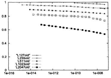
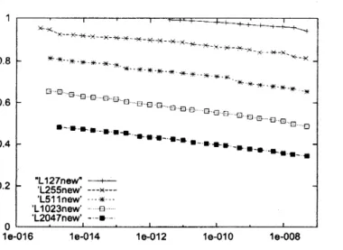
Figure 2: Relativecomputationalcosts of Legendre polynomial transforms by the old algorithm

Figures 2 and 3 show the floating point operation counts relative to the direct computation. The

x-axis shows the attained precision. $L12701d$” and _$Ll27new$” _{give the performances for $T=127$,}

etc.

Comparingthose figures,

we can see

that $T=127$ gives small difference between theold andthe

new

algorithms, but for $T=2047$ the old algorithm takes about 1.5 times $mo$

re

computations than

Figure 3: Relative computationalcosts of Legendre polynomialtransforms by the new algorithm

For the old algorithm, the gradient is different for$T=1023$with lower precision and for$T=2047$

thanthe other

cases.

This is becausethe split Legendre functionsare used only for those conditions.

However for the

new

algorithm, we found nosuch phase change.

Theplotsfor the old algorithm stop at precisionof$10^{-15}$ to$10^{-11}$. This isbecausehigher precision

was

not attained because of the numerical stability. For the new algorithm higher precisions

were

attained. Those results imply that the numerical stability is much improved in the

new

algorithm.

Further discussion on the performance will befound in [23].

5

Summary and future works

This paper discusses our fast algorithm for

as

sociated Legendre function transformswith generalized

FMM. This algorithm is formerly reported in

our

previous reports [22, 23], but the details of the

algorithmwerenotpresented. Inthis paper, the transform algorithm and the preprocessing algorithm

are

discussed. The performance is reported in English for the first time.

There

are

several remaining works to do.

The new algorithm performs better than the old algorithm, but its computational complexity is

not bounded theoretically. To bound it, the complexity bound for the interpolation with generalized

FMM must be obtained, and to that purpose,

we

must have some analytical expression for the

interpolation matrix entries.

Any specific property of the associated Legendre functions is utilized in the

new

algorithm.

The

new

algorithm just compresses the transform matrix. The only exception is that the forward

transformcan be obtained bytransposition ofthe inverse transform matrix, but this assumption

can

be removed if

we

compute the forward transform matrix directly. Thus the

new

algorithm

can

be

applied to any

_transform

at least conceptually.

Last, the implementation should be improved and released to the public use. Before doing that,

we

should improve the implementation of generalized FMM, because its current performance is

somewhat lower than theprevious one (but with dramatically reduced preprocessingtime).

Acknowledgments

This research is partly supported by Grant-in-Aid for Scientific Research

on

Priority Areas, MEXT

References

[1] B. K. Alpert and V. Rokhlin: A Fast Algorithm for the Evaluation of Legendre Expansions,

$SI\mathcal{A}M$J. Sci. Stat. Comput., Vol. 12, No. 1, pp. 158-179, 1991.

[2] G. Beylkin, R. R. Coifman, and V. Rokhlin: Fast WaveletTransformsandNumericalAlgorithms

I, Comm. Pure Appl. Math., No. 44, pp. 141-183, 1991.

[3] J. P. Bovd: Multipole expansions and pseudospectral cardinal functions: A

new

generation of

the fast Fourier transform, J. Comput. Phys., Vol. 103, pp. 184-186, 1992.

[4] A. Dutt, M. Gu, and V. Rokhlin: Fast algorithms for polynomial interpolation, integration, and

differentiation, SIAMJ. Numer. Anal., Vol. 33, No. 5, pp. 1689-1711, 1996.

[5] L. Greengard and V. Rokhlin: A Fast algorithm for particle simulations, J. Comput. Phys.,

Vol. 73, pp. 325-, 1987.

[6] J. R. Driscoll and D. Healy, Asymptotically Fast Algorithms for Spherical and Related

Trans-forms, Proc. 30th IEEE FOCS, pp. 344-349 (1989).

[7] D. M. Healy Jr., D. Rockmore, P. J. Kostelec, and S. S. B. Moore, FFTs for 2-Sphere –

Improvements and Variations, Tech. Rep. PCS-TR96-292, Dartmouth Univ., 1996.

[8] R. Jakob-Chien and B. K. Alpert, A Fast Spherical Filter with Uniform Resolution, J. Comput.

Phys., Vol. 136, pp. 580-584, 1997

[9] J. Keiner and D. Potts, Fast Evaluation of Quadrature Formulae

on

the Sphere, Math. Comp.,

Vol. 77, No. 261, pp. 397-419 (2008).

[10] S. Kunis and D. Potts, Fast spherical Fourier algorithms, J. Comp. Appl. Math., Vol. 161,

pp. 75-98 (2003).

[11] M. J. Mohlenkamp, A Fast Transform for Spherical Harmonics, J. Fourier Anal. Appl., Vol. 2,

pp. 159-184, 1999.

[12] A. Mori, R. Suda and M. Sugihara, An improvement on Orszag’s Fast Algorithm for Legendre

Polynomialhansform, Trans.

_Inform.

Process. Soc. Japan,Vol. 40, No. 9, pp. 3612-3615(1999).

[13] S. A. Orszag, Fast Eigenfunction T}ansforms, Science and Computers, Adv. Math.

Supplemen-tary Studies, Vol. 10, pp. 23-30, Academic Press, 1986.

[14] D. Potts, G. Steidl, and M. Tasche, Fast and stable algorithms for discrete spherical Fourier

transforms, Linear Algebra Appl., pp. 433–450, 1998.

[15] V. Rokhlin and M. Tygert: Fast algorithms for spherical harmonic expansions, SIAM J. Sci.

Comp. Vol. 27, No. 6, pp. 1903-1928 (2006).

[16] G. Szego, Orthogonal Polynomials, p. 193. AMS, 1959.

[17] R. Suda, A Fast SphericalHarmonics Transform Algorithm,

_Infor.

Proc. Soc. Japan SIGNotes,

No. 98-HPC-73, pp. 37-42, 1998.

[18] R. Suda: Stability Control ofFast Spherical Harmonics Transform,

_Info.

Proc. Soc. Japan SIG

Notes, No. 2001-HPC-88, pp. 43-48 (2001).

[19] R. Suda: Fast spherical harmonics transform of FLTSS and its evaluation, The 2002 Workshop

on

the Solution

_of

Panial

_Differential

Equations on the Sphere, Fields Inst., U. Toronto (2002).

[20] R. Suda: Fast spherical harmonic transform routine FLTSS applied to the shallow water test

set, Mon. Wea. Rev., Vol. 133, No. 3, pp. 634-648 (2005).

[21] R. Suda: Stabilityanalysis of the fast Legendre transform algorithm based

on

the fastmultipole

[22] R. Suda: Fast Spherical Harmonic Transform with generalized Fast Multipole Method, 2005

International

_Conference

on

_Scientific

Computing and

_Differential

Equations (SciCADE05),

p. 86 (2005)

[23] R. Suda: High Performance Implementation and Evaluation of the Spherical Harmonic

Trans-forms in the Fast Orthogonal Function Transform Routine FXTPACK,

_Info.

Proc. Soc. Japan

SIG Technical Report, Vol. 2005, No. 97 (2005-HPC-I04), pp. 31-36 (2005).

[24] R. Suda: FLTSS home page:

http:$//www$

.

na.

cse. nagoya-u. ac.$jp/\sim_{reiji}/fltss/$

[25] R. Suda and M. Takami: A Fast Spherical Harmonics Transform Algorithm, Math. Comp.,

Vol. 71, No. 238, pp. 703-715 (2002).

[26] R. Suda and M. Takami: Error Analysis and Control ofFast Spherical Harmonics Transform,

Info.

Proc.

Soc. Japan SIG Notes, No. 2000-HPC-84, pp. 7-12 (2000).

[27] R. Suda and M. Takami: Error Analysis and Control ofFast Spherical Harmonics Transform,

Tmns.

_Info.

Proc. Soc. Japan HPS, Vol. 42, No. SIG12 (HPS4), pp.49-59 (2001).

[28] R. Suda and S. Kuriyama: Another Preprocessing Algorithm for Generalized One-Dimensional

Fast Multipole Method, J. Comp. Phys., Vol.195, pp. 790-803 (2004).

[29] N. Yarvinand V. Rokhlin: A Generalized One-Dimensional Fast Multipole Method with