九州大学学術情報リポジトリ
Kyushu University Institutional Repository
反応拡散方程式系におけるパターン形成に対する計 算機援用証明
蔡, ??
九州大学大学院数理学府
https://doi.org/10.15017/21706
出版情報:Kyushu University, 2011, 博士(数理学), 課程博士 バージョン:
権利関係:
A computer-assisted proof for the pattern formation on reaction-diffusion systems
Shuting Cai
Graduate School of Mathematics, Kyushu University
2012
Contents
Abstract ii
1 Introduction 1
2 Some notations and projection error estimation 3
3 Approximate solution 17
4 Verification 21
4.1 Fixed point equation . . . 21
4.2 Verification condition . . . 22
4.2.1 Finite dimensional part . . . 23
4.2.2 Infinite dimensional part . . . 29
4.2.3 Verification Algorithm . . . 34
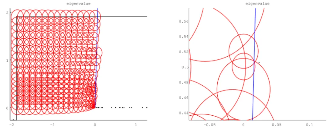
5 Eigenvalue excluding 37 5.1 Eigenvalue excluding theorem . . . 37
5.2 Invertibility condition of ˆL . . . 38
5.3 Computable criterion for the invertibility of ˆL . . . 41
5.4 Direct computation of upper bound for ˆL−1 . . . 48
5.5 Eigenvalue problem of the linearized operator at the exact solution . . . 51
6 The domain of attraction 56
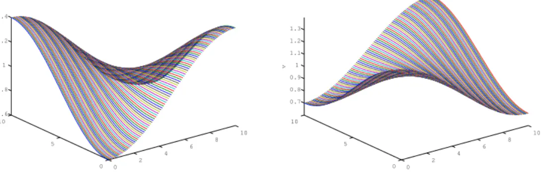
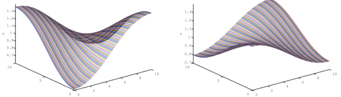
7 Numerical Results 63
8 Conclusions 67
Acknowledgements 68
References 69
Abstract
In this paper we give a method by computer-assistance to prove a pattern formation. As a typical model we consider two dimensional time-dependent reaction-diffusion equations with Neumann boundary conditions. For suit- able system parameters we solve (approximately) the parabolic problem, hop- ing for some convergence to some pattern formation stationary (approximate) solution, and improve the approximation to a stationary solution by Newton’s method, then enclose the stationary solution by our numerical verification method. Next we prove that the operator linearized at the exact stationary solution is a sectorial operator and compute a bound for the resolvent of the linearized operator which is needed for semigroup estimates. By using the semigroup estimate we analytically compute a domain of attraction for the stationary solution, i.e. some (norm-)neighborhood of the stationary solution such that, for initial data within this neighborhood, the parabolic solution converges to the stationary solution. For suitable initial conditions, if we enclose the solution of the parabolic problem until, for some time T, the en- closing set is a subset of the domain of attraction, then we can conclude that from time T on, convergence to the stationary solution takes place. This gives a complete convergence result, proving a pattern formation, for the initial conditions used for the parabolic problem.
Keyword:
Pattern formation; Computer-assisted proof; Reaction-diffusion system;
Domain of attraction.
Chapter 1 Introduction
We consider a time-dependent reaction-diffusion system with Neumann bound-
ary conditions
ut=γf(u, v) + ∆u in Ω, vt=γg(u, v) +d∆v in Ω,
∂u
∂ν = ∂v
∂ν = 0 on∂Ω,
(1.0.1)
where Ω is a bounded domain in ℜ2, γ, dare some positive constants,f, g are nonlinear/linear functions depending on each model and ν = (ν1, ν2) is an outer unit normal vector on ∂Ω.
This kind of problem (1.0.1) can be applied in mathematical biology[10, 11]. One simple system is FitzHugh-Nagumo reaction[6, 15]. In [7], u as an activator and v as an inhibitor are interpreted as relative concentrations of two substances known as morphogens. In [26], this kind of problem, called
”Excitable media”, can be applied in mammalian heart muscle and its cells and Xenopus eggs. For more background, see references in [23].
There are many papers considering the stationary solution of the system.
Here we mention some results on the systems of FitzHugh-Nagumo type.
There are several results about Dirichlet problem[4, 3, 20, 24]. In [4] the minimization problem associated with the system is considered, and in [3]
the peak solutions for the system are investigated. There is also one paper considering the relationship between the parameter and the solution of the system[20]. In [24], by using a numerical verification method, the author encloses the exact solution of the equations. There are also some results for Neumann problem. In [5] some results on the solutions with interior and boundary peaks are shown, and in [21] the relationship between one param- eter and the energy minimizers is discussed. In [2], the authors proposed a numerical verification method to enclose a solution of the two dimensional
system.
In this paper, we will propose a computer-assisted method to prove a pattern formation. Knowing the pattern formation is very important in biology[11]. When we solve a time-dependent problem, we often see some numerical convergence of them, but analytically there is no proof of it. On the other hand when we compute a steady state problem, we do not know from which initial state the stationary solution appeared. This paper is about how to overcome these two difficulties. As a concrete example, we will apply our method to Schnakenberg equation, which is another reaction-diffusion system.
There are eight chapters in this paper. In chapter 2, we prepare some function spaces and notations and then the fixed-point formulation and the construction of a priori error estimate for the projection are derived. And in Chapter 3, for suitable system parameters we solve (approximately) the parabolic problem and improve the approximation to a stationary (approxi- mate) solution by Newton’s method. After that, in Chapter 4, we use Nakao’s method to enclose the stationary solution near this approximate solution.
This method, which is similar to the method in [2], is based on the infi- nite dimensional fixed point theorem. First, the time-independent system is rewritten in a fixed point form and then the fixed point equation is decom- posed into the finite dimensional part and the infinite dimensional error part.
Based on these two parts, we construct a set which satisfies the hypothesis of Schauder’s fixed point theorem for a compact map in a suitable Sobolev space. This verification method was originated by Nakao[16] and then has been developed by him and his coworkers[18, 19, 12, 13, 14].
Then we prove that the operator linearized at the exact stationary so- lution is a sectorial operator and compute a bound for the resolvent of the linearized operator which is needed for semigroup estimates. By using the semigroup estimate we analytically compute a domain of attraction for the stationary solution. And thus, for suitable initial conditions, if we enclose the solution of the parabolic problem until, for some time T, the enclosing set is a subset of the domain of attraction, then we can conclude that from timeT on, convergence to the stationary solution takes place. This is showed in Chapter 6. And in order to get the results in Chapter 6, we propose a computer-assisted method to exclude the eigenvalues of the linearized oper- ator in Chapter 5. In Chapter 7, there are some numerical results. We apply our method to an example with some suitable system parameters and then get its domain of attraction. At last there are some conclusions in Chapter 8.
Chapter 2
Some notations and projection error es- timation
We consider the domain Ω = (0, l)×(0, l) ⊂ ℜ2(l ≥ 1). Then we choose basis function as
φi1i2(x, y) = cos(i1πx/l) cos(i2πy/l), i1, i2 = 0,1,2, . . . For a fixed non-negative integer N we reorder the basis function
φi = cos(i1πx/l) cos(i2πy/l),(i= 1,2,3,· · ·(N + 1)2) (i1, i2 = 0,1,2,· · ·N) in the following way:
i=i1(N + 1) +i2+ 1.
The Sobolev spaceWk,p(Ω)(1≤p≤+∞) is defined as Wk,p(Ω) :={u∈Lp(Ω) :Dαu∈Lp(Ω),∀|α| ≤k},
where α is a multi-index. The natural number k is called the order of the Sobolev space Wk,p(Ω).
And we suppose that for the L2-Sobolev space of order k on Ω, Hk(Ω), ψ ∈Hk(Ω) (k ≥0) is expanded in the Fourier series as
ψ =
∑∞ i=1
aiφi (ai ∈ ℜ).
For a non-negative integerN, let XN denote a function space as XN :=
{ vN =
∑N n,m=0
cnmφnm|cnm∈ ℜ }
⊂H2(Ω)⊂H1(Ω).
Forz1, z2 ∈H1(Ω), define the usual inner product as
⟨z1, z2⟩H1(Ω):= (z1, z2)L2(Ω)+ (∇z1,∇z2)L2(Ω), where (·,·)L2(Ω) means the inner product on L2(Ω).
Forz ∈Hk(Ω)(1≤k < ∞, k̸= 2), define the usual norm as
∥z∥2Hk(Ω) := ∑
|α|≤k
∥Dαz∥2L2(Ω).
When k= 2, for z = ∑∞
n,m=0
cnmφnm ∈H2(Ω), we have
∥z∥2L2(Ω)+∥∇z∥2L2(Ω)+∥∆z∥2L2(Ω)
=∥z∥2L2(Ω)+∥∇z∥2L2(Ω)+
∑∞ n,m=0
c2nm(∥(φnm)xx∥2L2(Ω)+∥(φnm)yy∥2L2(Ω) + 2((φnm)xx,(φnm)yy)L2(Ω))
=∥z∥2L2(Ω)+∥∇z∥2L2(Ω)+
∑∞ n,m=0
c2nm((n4+m4)π4/l4 + 2n2m2π4/l4)∥φnm∥2L2(Ω)
=∥z∥2L2(Ω)+∥∇z∥2L2(Ω)+
∑∞ n,m=0
c2nm(∥(φnm)xx∥2L2(Ω)+∥(φnm)yy∥2L2(Ω) + 2((φnm)xy,(φnm)xy)L2(Ω))
= ∑
|α|≤2
∥Dαz∥2L2(Ω),
where (φnm)x is the derivative of φnm with respect to x, (φnm)xy is the derivative of (φnm)x with respect to y and (φnm)xx, (φnm)yy are the second derivative of φnm with respect to x and y respectively, therefore, we define the norm in H2(Ω) as
∥z∥2H2(Ω):=∥z∥2L2(Ω)+∥∇z∥2L2(Ω)+∥∆z∥2L2(Ω). And for z1, z2 ∈H2(Ω), define the inner product as
⟨z1, z2⟩H2(Ω) := (z1, z2)L2(Ω)+ (∇z1,∇z2)L2(Ω)+ (∆z1,∆z2)L2(Ω). For z ∈ H1(Ω), let PN : H1(Ω) →XN denote the H1-projection defined by the truncation operator:
PN
( ∑∞
n,m=0
cnmφnm )
=
∑N n,m=0
cnmφnm,
which satisfies
⟨z−PNz, zN⟩H1(Ω) = 0, for all zN ∈XN. When z∈H2(Ω), we also have
⟨z−PNz, zN⟩H2(Ω) = 0, for all zN ∈XN. Therefore, we also use PN as a H2-projection.
Set P :H2(Ω)×H2(Ω)→XN ×XN as
P(z1, z2) := (PNz1, PNz2), z1, z2 ∈H2(Ω).
For Hilbert spaces X and Y, we define the inner product and the norm in X×Y as
(( x1 y1
) ,
( x2 y2
))
X×Y
:= (x1, x2)X + (y1, y2)Y
and
( x y
):=
√∥x∥2X +∥y∥2Y.
Defining the operator L : H2(Ω) → L2(Ω) by Lψ := −△ψ +ψ, we get the following lemma.
Lemma 2.0.1 For all ϕ∈L2(Ω), the linear equation { Lψ =ϕ in Ω,
∂ψ
∂ν = 0 on ∂Ω (2.0.1)
has the unique solution ψ ∈H2(Ω).
Proof. Let ψ = ∑∞
n,m=0
ψnmφnm (ψnm∈ ℜ, n, m= 0,1,2, . . .).
Forϕ= ∑∞
n,m=0
ϕnmφnm ∈L2(Ω) (ϕnm ∈ ℜ, n, m= 0,1,2, . . .),let
ψnm = ϕnm
1 +n2π2/l2+m2π2/l2, then Lψ =ϕ holds. By observing
∑∞ n,m=0
(1 +n2π2/l2+m2π2/l2 +n4π4/l4+m4π4/l4+ 2n2m2π4/l4)ψnm2
=
∑∞ n,m=0
(1 +n2π2/l2+m2π2/l2+n4π4/l4+m4π4/l4+ 2n2m2π4/l4)
·
( ϕnm
1 +n2π2/l2+m2π2/l2 )2
<
∑∞ n,m=0
3(l2+n4π4/l2+m4π4/l2) ϕ2nm
1 +n4π4/l4+m4π4/l4
=
∑∞ n,m=0
3ϕ2nml2 <∞, and
∥ψ∥2H2(Ω)
=
∑∞ n,m=0
(1 +n2π2/l2+m2π2/l2+n4π4/l4+m4π4/l4+ 2n2m2π4/l4)ψ2nm∥φnm∥2L2(Ω)
<
∑∞ n,m=0
l2(1 +n2π2/l2+m2π2/l2+n4π4/l4+m4π4/l4+ 2n2m2π4/l4)ψnm2 , ψ ∈H2(Ω) follows.
Noting that the solution ofLψ =ϕ is characterized as the solution of
∫
Ω
∇ψ· ∇v dx+
∫
Ω
ψv dx=
∫
Ω
ϕv dx, ∀v ∈H1(Ω),
we have ∫
Ω
(−∆ψ+ψ)v dx+
∫
∂Ω
∂ψ
∂νv dx=
∫
Ω
ϕv dx,
and thus ∫
∂Ω
∂ψ
∂νv dx= 0.
Sincev is arbitrary inH1(Ω), in case ψ ∈H2(Ω) we have ∂ψ∂ν = 0 in the trace sense.
If there exists another solution ˜ψ ̸=ψ, we get Lψ˜=ϕ,
which means the existence of a non-trivial solution of the equation Lφ= 0.
But noting that
(Lφ, φ)L2(Ω) =∥φ∥2H1(Ω)
holds, Lφ = 0 derives ∥φ∥2H1(Ω) = 0, i.e. φ = 0, which contradicts the assumption and the uniqueness of the solution of Lψ =ϕ follows. 2
Remark 2.0.2 For ϕ ∈ L2(Ω), we denote the solution of (2.0.1) as L−1ϕ.
Then it is clear that L−1ϕ satisfies Neumann boundary conditions.
Lemma 2.0.3 For all ϕ∈L2(Ω), the linear equation
(∆2−∆ +I)ψ =ϕ in Ω,
∫
∂Ω
(∂ψ
∂νv−∆ψ∂v
∂ν +∂(∆ψ)
∂ν v )
dx= 0, for ∀v ∈H2(Ω) has the unique solution ψ ∈H4(Ω).
Proof. Let ψ = ∑∞
n,m=0
ψnmφnm (ψnm∈ ℜ, n, m= 0,1,2, . . .).
Forϕ= ∑∞
n,m=0
ϕnmφnm ∈L2(Ω) (ϕnm ∈ ℜ, n, m= 0,1,2, . . .),let
ψnm= ϕnm
1 +n2π2/l2+m2π2/l2+n4π4/l4+m4π4/l4+ 2n2m2π4/l4, then (∆2−∆ +I)ψ =ϕ holds. By observing
∑∞ n,m=0
(1 +n2π2/l2+m2π2/l2+n4π4/l4+m4π4/l4+n6π6/l6+m6π6/l6 +n8π8/l8+m8π8/l8+ 2m2n2π4/l4+ 3m4n2π6/l6+ 3m2n4π6/l6
+ 4m2n6π8/l8+ 4n2m6π8/l8+ 6n4m4π8/l8)ψ2nm
=
∑∞ n,m=0
(1 +n2π2/l2+m2π2/l2+n4π4/l4+m4π4/l4+n6π6/l6+m6π6/l6 +n8π8/l8+m8π8/l8+ 2m2n2π4/l4+ 3m4n2π6/l6+ 3m2n4π6/l6
+ 4m2n6π8/l8+ 4n2m6π8/l8+ 6n4m4π8/l8)
·
( ϕnm
1 +n2π2/l2+m2π2/l2+n4π4/l4+m4π4/l4+ 2n2m2π4/l4 )2
<
∑∞ n,m=0
16(l4+n8π8/l2 +m8π8/l2) ϕ2nm
1 +n8π8/l8+m8π8/l8
=
∑∞ n,m=0
16ϕ2nml4 <∞,
and
∥ψ∥2H4
=
∑∞ n,m=0
(1 +n2π2/l2+m2π2/l2+n4π4/l4+m4π4/l4+n6π6/l6+m6π6/l6 +n8π8/l8+m8π8/l8+ 2m2n2π4/l4+ 3m4n2π6/l6+ 3m2n4π6/l6
+ 4m2n6π8/l8+ 4n2m6π8/l8+ 6n4m4π8/l8)ψ2nm∥φnm∥2L2
<
∑∞ n,m=0
l2(1 +n2π2/l2+m2π2/l2+n4π4/l4+m4π4/l4+n6π6/l6+m6π6/l6 +n8π8/l8+m8π8/l8+ 2m2n2π4/l4+ 3m4n2π6/l6+ 3m2n4π6/l6
+ 4m2n6π8/l8+ 4n2m6π8/l8+ 6n4m4π8/l8)ψ2nm, ψ ∈H4(Ω) follows.
Noting that the solution of (∆2 −∆ +I)ψ = ϕ is characterized as the solution of
∫
Ω
∆ψ∆v dx+
∫
Ω
∇ψ· ∇v dx+
∫
Ω
ψv dx=
∫
Ω
ϕv dx, ∀v ∈H2(Ω), we have
∫
Ω
(∆2ψ−∆ψ+ψ)v dx+
∫
∂Ω
∂ψ
∂νv dx+
∫
∂Ω
∂(∆ψ)
∂ν v dx−
∫
∂Ω
∂v
∂ν∆ψ dx=
∫
Ω
ϕv dx, and thus
∫
∂Ω
∂ψ
∂νv dx+
∫
∂Ω
∂(∆ψ)
∂ν v dx−
∫
∂Ω
∂v
∂ν∆ψ dx= 0.
If there exists another solution ˜ψ ̸=ψ, we get (∆2−∆ +I) ˜ψ =ϕ,
which means the existence of a non-trivial solution of the equation (∆2 −
∆ +I)φ= 0. But noting that
((∆2−∆ +I)φ, φ)L2(Ω)=∥φ∥2H2(Ω)
holds, (∆2−∆ +I)φ= 0 derives∥φ∥2H2(Ω) = 0, i.e. φ= 0, which contradicts the assumption and the uniqueness of the solution of (∆2 −∆ +I)ψ = ϕ follows. 2
Now we derive an estimation for the projection PN, an imbedding con- stant from H1(Ω) toLp(Ω) for 2≤p <∞ and an imbedding constant from H2(Ω) to Lp(Ω) for 2≤p≤ ∞.
Lemma 2.0.4 For all z ∈H4(Ω), we have
∥z−PNz∥H2(Ω) ≤C2(N)∥△2z− △z+z∥L2(Ω), where C2(N) = √
1
1+(N+1)2π2/l2+(N+1)4π4/l4. And for z∈H2(Ω),
∥z−PNz∥L2(Ω) ≤C2(N)∥z−PNz∥H2(Ω)
holds.
Proof. For z = ∑∞
n,m=0
cnmφnm ∈H2(Ω), we obtain
∥z−PNz∥2H2(Ω)
≤∥z−PNz∥2L2(Ω)+∥(z−PNz)x∥2L2(Ω)+∥(z−PNz)y∥2L2(Ω)+∥(z−PNz)xx∥2L2(Ω)
+∥(z−PNz)yy∥2L2(Ω)+ 2((z−PNz)xx,(z−PNz)yy)L2(Ω)
=
∑∞ n=N+1
∑∞ m=0
c2nm∥φnm∥2L2(Ω)+
∑N n=0
∑∞ m=N+1
c2nm∥φnm∥2L2(Ω)
+
∑∞ n=N+1
∑∞ m=0
c2nm∥(φnm)x∥2L2(Ω)+
∑N n=0
∑∞ m=N+1
c2nm∥(φnm)x∥2L2(Ω)
+
∑N n=0
∑∞ m=N+1
c2nm∥(φnm)y∥2L2(Ω)+
∑∞ n=N+1
∑∞ m=0
c2nm∥(φnm)y∥2L2(Ω)
+
∑∞ n=N+1
∑∞ m=0
c2nm∥(φnm)xx∥2L2(Ω)+
∑N n=0
∑∞ m=N+1
c2nm∥(φnm)xx∥2L2(Ω)
+
∑N n=0
∑∞ m=N+1
c2nm∥(φnm)yy∥2L2(Ω)+
∑∞ n=N+1
∑∞ m=0
c2nm∥(φnm)yy∥2L2(Ω)
+
∑N n=0
∑∞ m=N+1
c2nm2((φnm)xx,(φnm)yy)L2(Ω)+
∑∞ n=N+1
∑∞ m=0
c2nm2((φnm)xx,(φnm)yy)L2(Ω)
=
∑N n=0
∑∞ m=N+1
c2nm(∥φnm∥2L2(Ω)+∥(φnm)x∥2L2(Ω)+∥(φnm)y∥2L2(Ω)+∥(φnm)xx∥2L2(Ω) +∥(φnm)yy∥2L2(Ω)+ 2((φnm)xx,(φnm)yy)L2(Ω)) +
∑∞ n=N+1
∑∞ m=0
c2nm(∥φnm∥2L2(Ω)
+∥(φnm)x∥2L2(Ω)+∥(φnm)y∥2L2(Ω)+∥(φnm)xx∥2L2(Ω)+∥(φnm)yy∥2L2(Ω)
+ 2((φnm)xx,(φnm)yy)L2(Ω))
≤ ∑∞
n=N+1
∑∞ m=0
c2nm(1 +n2π2/l2+m2π2/l2+n4π4/l4+m4π4/l4+ 2n2m2π4/l4)∥φnm∥2L2(Ω)
+
∑N n=0
∑∞ m=N+1
c2nm(1 +n2π2/l2+m2π2/l2+n4π4/l4+m4π4/l4+ 2n2m2π4/l4)∥φnm∥2L2(Ω)
≤ 1
1 + (N + 1)2π2/l2+ (N + 1)4π4/l4
·
∑∞ n=0
∑∞ m=0
(1 +n2π2/l2+m2π2/l2+n4π4/l4+m4π4/l4 + 2n2m2π4/l4)2c2nm∥φnm∥2L2(Ω)
= 1
1 + (N + 1)2π2/l2+ (N + 1)4π4/l4∥∆2z−∆z+z∥2L2(Ω). So we get C2(N) =
√ 1
1+(N+1)2π2/l2+(N+1)4π4/l4.
For ∥z − PNz∥L2, we use the so-called Aubin-Nitsche technique. We consider the linear equation:
(∆2−∆ +I)Φ =z−PNz in Ω,
∫
∂Ω
(∂Φ
∂νv−∆Φ∂v
∂ν +∂(∆Φ)
∂ν v )
dx= 0,for ∀v ∈H2(Ω).
By Lemma 2.0.3, we know that there exists the unique solution Φ∈H4(Ω).
Therefore, we have
∥z−PNz∥2L2(Ω)
=(z−PNz, z−PNz)L2(Ω)= (z−PNz,(∆2−∆ +I)Φ)L2(Ω)
=(z−PNz,Φ)L2(Ω)+ (∇(z−PNz),∇Φ)L2(Ω)+ (∆(z−PNz),∆Φ)L2(Ω)
−
∫
∂Ω
(∂Φ
∂ν(z−PNz)−∆Φ∂(z−PNz)
∂ν + ∂(∆Φ)
∂ν (z−PNz) )
dx
=⟨z−PNz,Φ⟩H2(Ω)
=⟨z−PNz,Φ−PNϕ⟩H2(Ω)
≤∥z−PNz∥H2(Ω)∥Φ−PNΦ∥H2(Ω)
≤∥z−PNz∥H2(Ω)C2(N)∥z−PNz∥L2(Ω).
So ∥z−PNz∥L2(Ω) ≤C2(N)∥z−PNz∥H2(Ω) holds. 2
Lemma 2.0.5 Ω = (a, b)×(a, b), a < b. Then, for all u∈H1(Ω), we have
∥u∥Lp(Ω) ≤Kp∥u∥H1(Ω),(2≤p <∞) where Kp =
( 1
b−a +2√p2
)(p−2)/p
.
Proof. For (x, y)∈Ω, we have (x−a)|u(x, y)|p/2 =∫x
a
∂
∂t[(t−a)|u(t, y)|p/2]dt
=∫x
a |u(t, y)|p/2dt+p2∫x
a(t−a)|u(t, y)|p/2−2u(t, y)∂u∂x(t, y)dt
≤∫x
a |u(t, y)|p/2dt+ p2(b−a)∫x
a |u(t, y)|p/2−1∂u
∂x(t, y)dt, (2.0.2) and
(b−x)|u(x, y)|p/2 =−∫b x
∂
∂t[(b−t)|u(t, y)|p/2]dt
=∫b
x |u(t, y)|p/2dt− p2∫b
x(b−t)|u(t, y)|p/2−2u(t, y)∂u∂x(t, y)dt
≤∫b
x|u(t, y)|p/2dt+p2(b−a)∫b
x |u(t, y)|p/2−1∂u
∂x(t, y)dt.
(2.0.3) Adding (2.0.2) and (2.0.3), we get
(b−a)|u(x, y)|p/2 ≤∫b
a |u(t, y)|p/2dt+p2(b−a)∫b
a |u(t, y)|p/2−1∂u
∂x(t, y)dt
=:f(y).
(2.0.4) Analogously, integrating instead in y-direction,
(b−a)|u(x, y)|p/2 ≤∫b
a |u(x, t)|p/2dt+p2(b−a)∫b
a |u(x, t)|p/2−1∂u∂y(t, y)dt
=:g(x)
(2.0.5) holds.
Multiplying (2.0.4) and (2.0.5), we have
(b−a)2|u(x, y)|p ≤f(y)g(x) and integrating over Ω we obtain
(b−a)2
∫
Ω
|u(x, y)|pdxdy
≤
∫
Ω
f(y)g(x)dxdy = (∫ b
a
f(y)dy
) (∫ b a
g(x)dx )
= (∫
Ω
|u(t, y)|p/2dtdy+ p
2(b−a)
∫
Ω
|u(t, y)|p/2−1 ∂u
∂x(t, y) dtdy
)
· (∫
Ω
|u(x, t)|p/2dxdt+p
2(b−a)
∫
Ω
|u(x, t)|p/2−1 ∂u
∂y(x, t) dxdt
)
≤
∫
Ω
|u|p/2dxdy+p
2(b−a) (∫
Ω
|u|p−2dxdy
)1/2(∫
Ω
∂u
∂x
2dxdy
)1/2
·
∫
Ω
|u|p/2dxdy+p
2(b−a) (∫
Ω
|u|p−2dxdy
)1/2(∫
Ω
∂u
∂y
2dxdy )1/2
and thus, using (A +Bλ)(A+ Bµ) = A2 +AB(λ +µ) +B2λµ ≤ A2 +
√2AB√
λ2+µ2+12B2(λ2+µ2) = (A+√1 2B√
λ2+µ2)2, we have (b−a)2
∫
Ω
|u(x, y)|pdxdy
≤ (∫
Ω
|u|p/2dxdy+ p 2√
2(b−a) (∫
Ω
|u|p−2dxdy
)1/2(∫
Ω
|∇u|2dxdy
)1/2)2
i.e. we obtain
∫
Ω
|u|p ≤ (
1 b−a
∫
Ω
|u|p/2+ p 2√
2 (∫
Ω
|u|p−2
)1/2(∫
Ω
|∇u|2
)1/2)2
, (2.0.6) here and in the following we omit to write dxdy.
When p= 4, from (2.0.6), we have
∫
Ω|u|4 ≤(
b−a1
∫
Ω|u|2+√ 2(∫
Ω|u|2)1/2(∫
Ω|∇u|2)1/2)2
≤(
1 b−a
∫
Ω|u|2+√22(∫
Ω|u|2+∫
Ω|∇u|2))2
≤(
1 b−a +√22
)2(∫
Ω|u|2+∫
Ω|∇u|2)2
= ( 1
b−a+ √22 )2
∥u∥4H1(Ω),
therefore, for 2≤p < 4 by using H¨older’s inequality, we get
∫
Ω|u|p =∫
Ω|u|4−p|u|2p−4 ≤(∫
Ω|u|2)(4−p)/2(∫
Ω|u|4)(p−2)/2
≤ ∥u∥4H−1p(Ω)((
1 b−a+ √22
)2
∥u∥4H1(Ω)
)(p−2)/2
≤(
1 b−a +√22
)p−2
∥u∥pH1(Ω), that is,
∥u∥Lp(Ω) ≤ (
1 b−a +
√2 2
)(p−2)/p
∥u∥H1(Ω) (2≤p <4) (2.0.7)