under Uncertain Network
Conditions
Ravindra Sandaruwan Ranaweera
Department of Computer and Network Engineering
The University of Electro-Communications
A thesis submitted for the degree of
Doctor of Philosophy
APPROVED BY SUPERVISORY COMMITTEE:
Chairperson: Prof. Kitsuwan Nattapong
Member: Prof. Naoto Kishi
Member: Prof. Yasushi Yamao
Member: Prof. Eiji Oki
Member: Prof. Minoru Terada
ネットワーク状態には、トラフィック要求、ネットワークデバイスまたはリンクの 障害、およびノード負荷が含まれている。ユーザーが満足するサービスを提供しながら良好 なサービス品質を達成するためには、ロバスト的かつ効率的な経路を選択する必要がある。 本論文は、不確実なネットワーク条件でロバストな経路選択方式を提供する手法を 提案する。具体的には、トラフィック需要とリンク障害の不確定性を持つインターネットプ ロトコル(IP)ネットワークのためのリンク重み計算方式と、ノード負荷を考慮した経路選 択方式について提案する。また、それぞれ提案方式の効果をシミュレーション・実験を用い て確認し、最後に論文のまとめと今後展望について説明する。
Abstract
The constant evolution of network technologies pose a challenge in network performance management due to complicated and uncer-tain network conditions. Network conditions include traffic demand, failures in network devices or links, and node load. In order to achieve a desired quality of service while providing a satisfying service to cus-tomers, networks must be able to select paths robustly and efficiently. This thesis provides robust path selection schemes under uncertain network conditions. This thesis focuses on the uncertain network conditions of traffic demands, link failures, and node load, since they strongly affect network services.
In the first part of the thesis, a path selection scheme for Internet Protocol (IP) networks with traffic demand and link failure uncer-tainty is presented. Open Shortest Path First (OSPF) is widely used as a routing protocol in IP networks. OSPF selects the shortest path between source and destination pairs. To determine shortest paths, OSPF requires to assign link weight for each link in the network. If link weights are not optimal, network traffic may concentrate to one link and it may increase the packet drop rate, reducing the quality of service. Implementing the most appropriate set of link weights is a challenging traffic engineering problem in OSPF networks.
Start-time Optimization (SO) is a commonly used link weights optimization scheme. However, it does not consider network condi-tion changes caused by network failures, such as link failure, nor traffic demand changes. Preventive Start-time Optimization (PSO) on the other hand considers network changes caused by link failures preven-tively and calculates an optimal set of link weights. SO and PSO
task for network operators. These link weight optimization methods may not be fully applicable in a context where the traffic demand often fluctuates. In order to handle traffic demand fluctuations dy-namically, the path selection scheme presented in this thesis uses a so-called hose model. In the hose model, specifying the total egress and ingress traffic at each node is enough; a traffic demand between each source and destination pair is not required to be specified.
Network operators may have different objectives when configuring routing paths. One network operator may want to configure paths to reduce the network congestion. Another network operator may want to configure paths to reduce the network resource usage. In order to address these objectives, the path selection scheme presented in this thesis is applied to reduce the network congestion and the network resource usage. The network congestion reduction and the network resource reduction problems are formulated as mixed integer linear programming (MILP) problems that consider both traffic demand fluctuation and link failure. To mitigate the complexity of solving the MILP formulations, heuristic approaches are also presented. Sim-ulation results show that the presented scheme, while being robust to traffic demand fluctuations and link failures, is able to reduce the network congestion and the network resource usage.
In the second part of the thesis, a path selection scheme for net-works considering node load is presented. A group of nodes or servers connected with links is also a network. In order to communicate be-tween servers in the network, a source server sends data packets to a destination server through the network and the destination server responds to the source server accordingly. As a consequence of the destination server being heavily loaded, data packets will be queued to be processed later making the response time longer. On the other hand, relatively free destination server will respond quickly finishing
the communication process in a shorter time. Therefore, response time or delay time between two servers can be used to measure server load.
Apache Hadoop (Hadoop) is a parallel-distributed computing framework and usually consists with tens to thousands of servers. These servers are connected via network to run jobs in a distributed manner. The storage layer of Hadoop, called Hadoop Distributed File System (HDFS) calculates paths between servers based on each server’s rack assignment information. Rack assignment is configured by the cluster administrator. HDFS keeps three (by default) or more replicas (copies) of each data block for fault tolerance and availabil-ity purposes. When a client wants to fetch non-local data, HDFS selects a server that holds a replica of that data based on the proxim-ity to the client. This source client and multiple destination servers that hold the data, result in multiple paths between the source and destinations. Selecting one destination server to fetch data from can also be said as selecting one path between the source and a destina-tion server. HDFS only considers the distance (hop count) between servers and does not consider server load of the destination when se-lecting a destination server. This hop count based static behavior of selecting a destination server decreases the overall efficiency of the cluster, wasting valuable cluster resources.
This thesis also presents a path selection scheme based on de-lay distribution between servers for Hadoop clusters. This scheme selects a destination server by comparing the delay distributions be-tween client-server pairs. The delay distributions are calculated by measuring the round-trip time between server pairs periodically. Our experiments observe that the presented scheme, while being robust to server load and network delay, is able to select the best path result-ing shorter data fetch time compared to conventional Hadoop. This reduction in data fetch time will lead to the reduction in job runtime,
Acknowledgements
This thesis is the summary of my doctoral study at the University of Electro-Communications, Tokyo, Japan. I am grateful to a large number of people who have helped me to accomplish this work.
First of all, I would like to express my sincere gratitude to my advisors, Professor Eiji Oki and Assistant Professor Nattapong Kit-suwan, for their mentor-ship, guidance and encouragements. Espe-cially, by working under the supervision of Professor Oki, I received an invaluable experience that helped me to shape my academic and professional skills.
I would like to thank my previous senior manager at work, Mr. Shuji Ushida for allowing me to start my doctoral study while working full-time at the company.
I would like to express my sincere appreciation to Professor Naoto Kishi, Professor Yasushi Yamao, and Professor Minoru Terada for be-ing part of my judgbe-ing committee and providbe-ing their precious com-ments to improve this thesis.
Finally, I want to deeply thank my lovely wife, parents, and friends for all the support and caring.
Contents
List of Figures v
List of Tables vii
1 Introduction 1
1.1 Uncertainty of network conditions . . . 1
1.2 Routing in IP networks . . . 4
1.3 Link weight optimization . . . 5
1.4 Traffic demand models . . . 7
1.5 Apache Hadoop . . . 8
1.6 Problem formulation . . . 11
1.6.1 Path selection scheme considering traffic demand and link failure uncertainty . . . 11
1.6.2 Path selection scheme considering node load uncertainty . 11 1.7 Contributions . . . 12
1.8 Organization of the thesis . . . 13
2 Path selection scheme for congestion reduction with link failure and traffic uncertainty 15 2.1 Network congestion . . . 15
2.2 Terminologies . . . 16
2.3 MILP formulation for congestion reduction . . . 18
2.4 Heuristic approach . . . 20
3 Path selection scheme for energy consumption reduction with
link failure and traffic uncertainty 35
3.1 Energy saving routing . . . 35
3.2 MILP formulation for energy consumption reduction . . . 37
3.3 Heuristic approach . . . 39
3.4 Simulation results . . . 39
3.5 Summary . . . 43
4 Path selection scheme for networks with imbalanced node load 47 4.1 Overview of Hadoop . . . 47
4.1.1 Components of Hadoop . . . 48
4.1.2 MapReduce framework . . . 50
4.1.3 Rack awareness . . . 51
4.1.4 Data read procedure in HDFS . . . 51
4.2 Path selection scheme under node load uncertainty . . . 53
5 Experimental results of path selection scheme for networks with imbalanced node load 59 5.1 Experiment environment . . . 59
5.2 Results and discussions . . . 60
5.3 Summary . . . 67
6 Conclusions and future works 69 6.1 Conclusions . . . 69
6.2 Future work . . . 71
References 73
List of Figures
1.1 A simple network topology and topologies after single link failure 6
1.2 Pipe model and its traffic demand . . . 8
1.3 Hose model and its traffic constraints . . . 8
1.4 Replica selection is equal to path selection . . . 10
1.5 Organization of the thesis . . . 14
2.1 Sample networks used in the simulations . . . 24
2.2 Random networks generated using BRITE . . . 30
2.3 α’s dependency on number of nodes and adjacency nodes . . . . . 31
2.4 β’s dependency on number of nodes and adjacency nodes . . . . . 32
3.1 α’s dependency on number of nodes and adjacency nodes . . . . . 42
3.2 β’s dependency on number of nodes and adjacency nodes . . . . . 43
4.1 Components of Hadoop and their relationship . . . 50
4.2 Fat tree topology based Hadoop cluster . . . 52
List of Tables
2.1 Characteristics of the sample networks used to compare the
heuris-tic and conventional schemes . . . 25
2.2 Comparison of worst-case network congestion ratios of MILP and the heuristic . . . 26
2.3 Comparison of worst-case network congestion ratios of the heuristic and conventional schemes for single link failure scenarios . . . 27
2.4 Comparison of network congestion ratios with no link failure . . . 28
2.5 Characteristics of the random sample networks . . . 29
2.6 Comparison of worst-case congestion ratios with different link weight setting schemes . . . 33
2.7 Comparison of presented scheme’s performance related to Ic . . . 33
2.8 Comparison of worst-case congestion ratios of ECMP routing and single path routing . . . 34
3.1 Comparison of worst-case network resource usage for any single link fail-ure scenario . . . 40
3.2 Comparison of network resource usage for no link failure scenario 41 3.3 Comparison of presented scheme’s performance related to Ic . . . 44
3.4 Comparison of worst-case resource usages of ECMP routing and single path routing . . . 44
5.1 Virtual server specifications . . . 61
5.2 Data fetch times of different ϵ values . . . . 61
5.3 HDFS data fetch times . . . 62
5.5 Wordcount job completion time without background jobs running 65 5.6 HDFS data fetch time with changing the number of background jobs 66 5.7 Comparison of data fetch time with fetched data size . . . 67
Chapter 1
Introduction
Communication networks (networks) play a critical role in modern software sys-tems. Routing is the main process used to send data from point A to point B by determining a path (route) that exists in the network [1]. In this thesis, the term
routing is used to refer sending data along the selected path. A stable network
is crucial for software systems to provide their intended services without any in-terruption. However, networks are inherently unpredictable requiring robust and efficient path selection schemes to provide satisfying services to customers.
Network instability is caused by a variety of factors; link failures, router fail-ures, traffic demand fluctuations, node overload, software configuration errors and bugs, malicious attacks, and human errors [1, 2, 7]. One or more of these problems affect the performance of the network. This thesis considers link failures, traffic demand fluctuations, and node load since they strongly affect network services and can be managed by routing schemes easily compared to others. Since router failures can be interpret as multiple link failures, malicious network attacks and errors related to software and human are unmanageable by routing schemes, they are considered as being out of scope of this work.
1.1
Uncertainty of network conditions
In general, a network consists with nodes and links. A link connects two nodes allowing them to exchange data between each other. Data that travel through the network is called traffic in general. A critical function of a network is to carry
traffic from one node to another based on routing decisions. Usually, routing decisions are dictated by the requirements of the network in addition to specific goals of a network service provider. Such goals may include how to provide an efficient and fair service so that most users receive an acceptable service rather than few specific users receiving outstanding service. Aforesaid view is partly required because there are finite amount of resources in a network, e.g., link capacity, and a service provider has a responsibility to treat all traffic neutrally [9].
The traffic volume that a source node requests to send to a destination node, is called a traffic demand in Internet Protocol (IP) networks. The set which describes all the demands between every source-destination pair in the network is called the traffic matrix. In real-world networks, traffic demand between all the source-destination node pairs can easily fluctuate. This makes it difficult for network operators or network administrators to know the actual traffic matrix, especially when the network size is large [8]. This uncertain nature of the traffic can impact the path selection decisions of the network adversely affecting the quality of service [1, 10, 11, 39]. Considering traffic demand uncertainty for design and planning of IP networks has recently attracted much attention [10, 11, 13, 14, 15, 40]. Bauschert et al. [10] presented multi-layer and mixed-line-rate network designs for network planning under traffic demand uncertainty. In [11], the authors considered the egress traffic demand at each node to calculate robust paths. Mitra et al. [12] presented a scheme to maximize the revenue under uncertain traffic demands. All of these work stress the importance of robust path selection schemes under uncertain traffic demands. Therefore, it is necessary to study ways to minimize the impact of traffic demand fluctuations.
Emerging software systems rely on the reliability of networks. Unfortunately, due to network failures such as link failures, maintenance windows, router reboots, etc. these services are adversely affected [17, 18]. Among these failures, link failures are considered to be one of the main challenges faced by network operators because link failures occur on a daily basis [17]. Moreover, it is observed that most of the link failures are common and transient. Failures in information networks are common and can result in substantial losses [19]. Recovery from link failures in IP networks can take a long time [21] because most of the IP
1.1 Uncertainty of network conditions
routing protocols are not designed to minimize network outages. In [21] it says that a single link failure can cause users to experience network service outages of several minutes even when the underlying network is highly redundant with plenty of spare bandwidth available and with multiple ways to route around the failure. Needless to say, depending on the application, outages of several minutes are not acceptable, for example, for e-commerce, voice over IP (VoIP) services, or transportation systems. Therefore, it is necessary to study ways to minimize the impact of link failures. For more information regarding the impacts of link failure, I would like to refer readers to [19, 20].
Depending on the type of the network, nodes have different names [1]. For example, routers, switches, servers etc. can be called nodes depending on the network type. Suppose that a source server communicate to a destination server and the destination server is overloaded. The destination server will queue the request to process later, making the response time longer. On the other hand, a relatively free destination server that can serve the source server’s request may respond without any delay. In distributed computing environments, node load becomes a key challenge in node selection [22]. Zhang et al. [23] presented an scheme that prevents node overload by delaying routing updates. Chang et al. [24] investigated the router performance of commercial routers depending on the workload. They found that some routers exhibit performance degradations in overloaded routers. Reference [1] explains the effects of routing instability caused by overloaded nodes. It also explains the impacts of “Network storm effect”, which is caused by overloaded nodes. In order to indicate that a router is in overloaded condition, a “overload bit” is used to communicate the overloaded situation to other routers. Sending excessive amount of state by one node to other nodes within the network, overloads the other nodes. This is considered a large threat to todays routing protocols [26]. Node overload can frequently lead to problems in queuing delay of data processing [2]. This delay caused by node overload can adversely affect the quality of service. Therefore, it is necessary to study ways to minimize the impact of node overload.
In recent years, the idea of robust optimization has gained much attention in the field of optimization [3, 4]. Robust optimization deals with uncertainty in the data of optimization problems. Under this framework, the objective and
constraint functions are only assumed to belong to certain sets in function space (the so-called “uncertainty sets”). The goal is to make a decision that is feasible no matter what the constraints turn out to be, and optimal for the worst-case objective function (min-max objective). Mulvey et al. [5] presented an approach that integrates goal programming formulations with scenario-based description of the problem data. Soyster [6] et al. presented a linear optimization model to construct a solution that is feasible for all input data such that each uncertain input data can take any value from an interval. Robust optimization is being used in many real-world applications such as finance, mechanics, and control etc. due to the recent progress in linear programming.
1.2
Routing in IP networks
Routing is the main process used to deliver data in networks. IP networks use hop-by-hop routing model. This means that each router is only responsible for for-warding a datagram to another router. This process continues until the datagram reaches its destination or times-out because its path is too long. Random-walk routing techniques are not particularly reliable, and so it is important that the routers in a network have a coordinated approach to decide which is the next hop along the path to a destination. Routing techniques essentially pass infor-mation between neighboring routers and use this data to build the shortest paths to all destinations. These are then stored in a routing table and passed on to the router’s neighbors. The path computation model deployed in IP networks is iterative and distributed.
These next hop information in the routing table can either be set manually or dynamically. In simple networks, routing tables can be manually configured or learned from the configuration of interfaces on the router [1]. In more complex networks in which there are many routers arranged in a mesh with lots of links between routers, each link having different capabilities, manual configuration be-comes onerous. More important - when a link or a router fails, all of the routing tables across the whole network must be updated to take account of the change. Similar changes are desirable when failures are repaired or when new links and
1.3 Link weight optimization
nodes are added. Therefore, it is desirable to use a routing protocol to determine the next hop information dynamically.
Open Shortest Path First (OSPF) [28] is a widely used protocol that routes IP packets dynamically. It gathers link state information from available routers and constructs a topology map of the network. The topology determines the routing table presented to the Internet Layer which makes the routing decisions based solely on the destination IP address found in IP packets. OSPF detects changes in the topology, such as link failures, very quickly and converges on a new loop-free routing structure within seconds using detour routes. It computes the shortest path tree for each route using a method based on Dijkstra’s algorithm [29], a shortest path first algorithm. In order to select a specific path in OSPF, there are costs assigned to all of the links. Traffic engineering is the process of predetermining the path through the network that various flows of data will travel and link cost (link weight) is used to introduce traffic engineering in OSPF routing model. Link weights must be calculated considering network topology, network resources etc. so that the calculated link weights would satisfy the requirements set by the network operator.
1.3
Link weight optimization
Based on weights of links in the network, routing protocols find the end-to-end path for each source-destination pair such that the sum of link weights on the path is minimized, so called the shortest path. Hence, to find a ‘good’ path for each source and destination pair that satisfies some network constraints such as the quality of service (QoS) of each session, energy consumption, and the target utilization of each link, it is important to assign the appropriate weight for each link in the network. A simple default weight setting policy suggested by Cisco [31] is to make the weight of a link inversely proportional to its capacity. But this simple weight setting policy do not emphasize on traffic matrix (traffic demand) or required traffic over link. So still this does not give the most optimal performance for the oblivious routing.
A more efficient way is optimizing link weights for a given topology consid-ering the traffic over the network which will reduce a certain objective function.
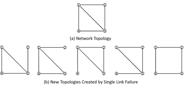
This scheme is called as Start-time Optimization (SO). Optimization provides network operators with a powerful method for traffic engineering. Its general objective is to distribute traffic flows evenly across available network resources in order to avoid network congestion and quality of service (QoS) degradation. Mul-tiple algorithms that focus on implementing SO are presented in [32, 33]. These studies all assume that the network topology and the traffic matrix are given. Unfortunately, SO is weak against link failures. When a link failure occurs, traf-fic related to that link should be re-routed through other active links, which can create an excess load to any other link and causes congestion in the network. Link failure is considered as a failure but if we consider it as a topology change in the network, we can take precautions for this problem in routing. When a link fails, the network takes a new shape. So we can take topology as a variable which can change with time because of link failure. For every possible link failure, we can get a new topology. If we consider a network topology as shown in Figure 1.1(a), all the new topologies created by single link failure will be shown as Figure 1.1(b).
Figure 1.1: A simple network topology and topologies after single link failure
The weakness of SO can be overcome by computing a new optimal set of link weights whenever the topology is changed. It can be said that this approach,
1.4 Traffic demand models
called Run-time Optimization (RO) provides the best routing performance after link failure. However, updating link weights in any case may lead to network instability [34] and 50% of link failures last less than one minute [17]. The analysis in [17] observed that more than 70% of transient failures that lasted less than 10 minutes are single link failures. Therefore, it seems reasonable to target the one-time configuration of link weights that can handle any single link failure.
PSO is a scheme that determines, at the start time, a suitable set of link weights that can handle any single link failure scenario preventively [35]. The ob-jective of this scheme is to determine, at the start time, the most appropriate set of link weights that can avoid both unexpected network congestion and network instability, the drawbacks of SO and RO, regardless of which link fails. PSO con-siders all possible single link failure scenarios at start time in order to determine a suitable set of link weights. However, the current PSO scheme is usable when the traffic demand of the network is exactly known. This traffic model is called a pipe model. However, in general, the pipe model is proved to be very difficult for network operators to use [36, 37, 38].
1.4
Traffic demand models
In terms of bandwidth specification, networks can be divided into a pipe model and a hose model. The pipe model needs to specify the traffic demand between any two nodes. It means that the entire traffic demand (traffic matrix) of the network is given [36, 37, 38]. Figure 1.2 shows an example of the pipe model and its traffic demand. Even though the pipe model generally achieves a high performance, it is difficult to measure or predict the traffic matrix in reality [37]. The PSO scheme [35] introduced in section 1.3 is based on the pipe model. It calculates an optimal link weight set that can handle single link failures assuming the traffic matrix is given.
Since the prediction of the actual traffic requirement as required in the pipe model is difficult, it is, therefore, considered to be easier for network operators to specify the traffic as just the total ingress (αi) and egress traffic (βi) (i.e., the amount of traffic that can be sent to and received from the backbone network) at each node. The traffic model that has achieved this specification is called
Figure 1.2: Pipe model and its traffic demand
a hose model [40]. An example of the hose model is shown in Figure 1.3. The ingress and egress bandwidth requirement is as Equation (1.1). Chu et al. formu-lated the general routing problem of the hose model and presented an algorithm for solving the link weight searching problem in [39]. The hose model presents some challenging problems for traffic engineering as the hose model only needs to specify the total ingress bandwidth requirement and the total egress bandwidth requirement at each node.
Figure 1.3: Hose model and its traffic constraints
∑ j dij ≤ αi (1.1a) ∑ i dij ≤ βj (1.1b)
1.5
Apache Hadoop
Apache Hadoop (Hadoop) [41], an open-source implementation of Google’s MapRe-duce [42] framework, is a parallel-distributed processing framework that allows
or-1.5 Apache Hadoop
ganizations to efficiently process very large datasets using commodity hardware in a realistic time. Hadoop has become the most popular parallel-distributed frame-work for processing large-scale data because it hides the complexity of distributed computing, scheduling, and communication while providing fault-tolerance. In general, Hadoop clusters are made with tens to thousands of servers. Hadoop makes use of inexpensive, industry standard commodity servers to store and pro-cess data rather than relying on specially built proprietary servers. Thus, most of the fortune 500 companies exploit Hadoop to process large-scale data within a reasonable budget. Initially, Hadoop was used at large companies such as Yahoo, Facebook, eBay etc., who already had large amounts of data and their Hadoop clusters are usually deployed in on-premise physical clusters.
HDFS (Hadoop Distributed File System) is the distributed storage layer that is responsible for storing data in Hadoop. Data in HDFS are broken into blocks and stored as replicas in multiple (at least three), different servers for fault-tolerance and availability purposes. Data processing tasks in Hadoop such as MapReduce jobs, Hive queries or Spark jobs access data stored in HDFS as re-quired by the task. HDFS is designed with write-once-read-many access model [43, 44] to attain high throughput of data access. Write-once-read-many means that once data is written to HDFS, that particular data will be read by processing tasks many times over the time. Therefore, improving how data is read in HDFS has a larger impact on the overall performance of HDFS compared to improving how data is written.
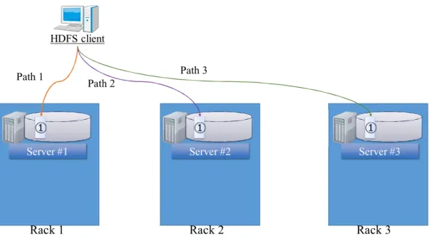
Let us consider how HDFS fetches (this thesis uses fetch in similar meaning to read since a client that wants to read data has to fetch data from a remote server) a particular data block in a high level. As we described earlier, there are three replicas of the same data block in three different servers. Therefore, HDFS has the freedom to select one of those servers when reading a particular data block. As shown in Figure 1.4, selecting one server is similar to selecting a path between two servers; if Server #1 is selected it is similar to selecting Path 1, if Server #2 is selected it is similar to selecting Path 2, and if Server #3 is selected it is similar to selecting Path 3. When there are three choices to select from, how HDFS chooses one among them is an interesting question. When fetching a data block, HDFS finds the best server to fetch data from by only comparing the network distance of
servers that hold a replica of the data block. The concept called “rack awareness” is used to calculate the network distance. We will explain “rack awareness” and how network distance is calculated in section 4.1 in detail. As we explained in section 1.1, server load is a major factor that should be considered when path selection decisions are made. However, HDFS does not consider the server load when selecting a server to fetch data from.
Figure 1.4: Replica selection is equal to path selection
There are multiple studies in literature that studied on improving resource management, job scheduling, and replica placement in Hadoop. Tan et al. studied analytical models for scheduling jobs based on extensive measurements and source code investigations [48]. Rasley et al. studied queue management techniques, such as appropriate queue sizing, prioritization of task execution via queue reordering, starvation freedom, and careful placement of tasks to queues [49]. Li et al. studied novel predictive scheduling framework to enable fast and distributed stream data processing [50]. Zaharia et al. addressed the problem of data locality while keeping fairness during task execution [51]. Many improvements for enhancing data placement (data write) in HDFS were studied in [70, 71, 72].
1.6 Problem formulation
1.6
Problem formulation
1.6.1
Path selection scheme considering traffic demand
and link failure uncertainty
OSPF is a widely used routing protocol in IP networks. OSPF requires link weights to be assigned to each link to calculate the shortest paths between every source-destination pair. In order to provide efficient routing to the users, these link weights must be calculated according to the network topology and service provider’s requirements. SO calculates an optimal set of link weights for a given topology when the exact traffic demand is known (pipe model) that will reduce a certain objective function, such as congestion ratio or energy consumption of the network. However, apart form the difficulty of exactly knowing the traffic demand, SO is weak against link failures and traffic demand fluctuations because it only considers one topology and one traffic pattern at a time. A scheme ap-plying the hose model, that can handle traffic demand fluctuations, on the other hand, provides robustness against traffic demand uncertainty. Chu et al. studied how to apply SO to the hose model. PSO on the other hand can calculate an optimal link weight set which is robust against link failures at start time if the traffic demand is exactly known. However, how to apply PSO for the hose model has not been studied. Being able to handle traffic demand fluctuations while guaranteeing robustness against link failure is desirable for network operators. This is the objective of the first part of this thesis.
1.6.2
Path selection scheme considering node load
uncer-tainty
Hadoop is an open-source parallel-distributed processing framework. Hadoop can efficiently use the resources of commodity servers that are connected to a network. The storage layer of Hadoop, called HDFS, stores data as blocks and each block is replicated to multiple servers for fault-tolerance and availability purposes. HDFS is designed with write-once-read-many access model meaning every improvement made to data reading mechanism contributes to improving overall performance of the cluster. When a client reads a data block, it has the choice of selecting
one server among the three servers that holds the same data block as replicas. HDFS selects a server to fetch data from considering the network distance and do not consider the server load of each server even though it affects the cluster performance. Therefore, robustness against server load in HDFS is desirable for Hadoop clusters. This is the objective of the second part of this thesis.
1.7
Contributions
This thesis proposes robust path selection schemes under uncertain network con-ditions. It presents a path selection scheme considering traffic demand and link failure uncertainty, and a path selection scheme considering server load uncer-tainty.
In the first part, path selection problem considering link failure under un-certain traffic conditions is studied. Robust optimization approach presented in this part is based on the hose model. In the hose model, contrary to the pipe model, the exact traffic matrix does not need to be specified by the network op-erators. The network operators can however set bounds on the total ingress and egress traffic at each node from their experience. Modeling the traffic for hose model allows an optimization scheme to accommodate any traffic matrix that fits within the bounds at each node. Link failures in a network can be considered as a topology change as we explained in section 1.3. We introduce a link weight optimization model for OSPF that takes traffic matrix and topology as variables. Usually, routing decisions are made to satisfy network operator’s objectives such as reducing the network congestion, reducing the energy consumption, sat-isfying the target link utilization of each link etc. We formulate mixed integer linear programming (MILP) problems to reduce worst-case network congestion and to reduce worst-case energy consumption by putting unnecessary links into sleep mode. Due to the complexity of solving the MILP formulations, we present heuristics to calculate a link weight set that achieves satisfactory performance in practical time. The heuristics consider the case traffic matrix and worst-case link failure topology to calculate a link weight set in practical time. Sim-ulation results observe that the presented schemes, while being robust to link
1.8 Organization of the thesis
failure and traffic demand fluctuation, is able to reduce the worst-case network congestion and worst-case energy consumption.
In the second part, a robust path selection problem considering node load is studied. In HDFS, rack information is used to calculate the network distance between servers notwithstanding the server load. This thesis presents a path selection scheme based on the delay distribution between servers for Hadoop clusters. This scheme calculates the round-trip time between all server pairs pe-riodically. The presented scheme selects a server comparing the delay distribution between server pairs. In order to achieve this, changes are made to source code of HDFS. Using the changed source code, we rebuilt Hadoop software packages and configured multiple Hadoop clusters to do experiments. The experiment results observe that the presented scheme, while being robust to server load, is able to dynamically select the best server resulting shorter data fetch time compared to conventional Hadoop.
1.8
Organization of the thesis
The organization of the thesis is shown in Figure 1.5. Path selection schemes considering traffic demand and link failure uncertainty is presented in chapter 2 to 3. Chapter 4 to 5 present path selection scheme considering server load uncertainty. Chapter 6 concludes the thesis.
A scheme to calculate a link weight set that is robust against link failure and traffic demand fluctuation, minimizing the worst-case network congestion is presented in chapter 2. Chapter 2 also includes the MILP formulation and simu-lation results. A scheme to calculate a link weight set that is robust against link failure and traffic demand fluctuation minimizing the worst-case network energy consumption is presented in chapter 3. It also includes the MILP formulation and simulation results.
A scheme to select paths considering server load is presented in chapter 4. Since experimental results have more impact than simulation results, experimen-tal environment information and results are introduced in chapter 5.
Chapter 2
Path selection scheme for
congestion reduction with link
failure and traffic uncertainty
Traffic engineering is the process of predetermining the paths through the network that various flow of data will travel. Link weight is used to introduce traffic engineering in OSPF routing model. A link weight calculation scheme that is optimized to achieve the objective(s) of network service providers is required. In this chapter, a path selection scheme that is robust against link failure and traffic demand fluctuation with the objective of reducing the worst-case congestion is presented. In section 2.1, network congestion and the importance of reducing network congestion is introduced. Terminologies used in the later sections are defined in section 2.2. In section 2.3, the MILP formulation to reduce the worst-case congestion ratio is introduced and the heuristic algorithm is introduced in section 2.4. Section 2.5 presents the simulation results.
2.1
Network congestion
Network congestion is the result of a route in the network being heavily utilized. Network congestion can deteriorate network service quality, resulting in queuing delay, data packet loss and the blocking of new connections [56]. Since, in OSPF,
routes are determined by link weights, link weights can be optimized so that each route in the network maintains a manageable congestion level.
One useful approach to enhance routing performance is to minimize the max-imum link utilization rate, network congestion ratio, of all links in the network. Reducing the congestion ratio in the network is a common objective of network service providers [1]. Also, they must be prepared for the worst-case scenario, worst-case congestion ratio, to maintain a satisfying service. Therefore, network service providers configure routes in the network to minimize the worst-case con-gestion ratio [57] increasing the admissible traffic [56].
2.2
Terminologies
The network is described as a directed graph G(V, E), where V is the set of nodes and E is the set of links. v ∈ V , where v = 1, 2, . . . , N, indicates an individual node and a link from node i∈ V to node j ∈ V is denoted as (i, j) ∈ E. N is the number of nodes and L is the number of links in the network, or L =|E|. cij is the capacity of link (i, j)∈ E. The traffic volume on link (i, j) ∈ E is denoted as uij. Since the probability of concurrent multiple link failures is much less than that of single link failures [17, 18], only single link failures in the network are considered in this study. F is the set of link failure indices l, where l = 0, 1, 2,· · · , L and
F = E∪ {0}. The number of elements in F is |F | = L + 1. l = 0 indicates no
link failure and l(̸= 0) indicates the failure of link (i, j) = l(̸= 0). The network in which lth (̸=0) link failed is described as a directed graph Gl(V, El). As G0(V, E0)
indicates no link failure, G0(V, E0) = G(V, E) and let ˜G be the set of network
topologies. cl
ij is the capacity of (i, j) ∈ El. If (i, j) = l, clij = 0. W = {wij} is the link weight matrix of network G, where wij is the weight of link (i, j). Let
{1, . . . , wmax} be the set of possible link weights. xpqij is the portion of traffic from node p ∈ V to node q ∈ V routed through (i, j) ∈ E. xpqij(W, l) is used to represent the load distribution variables under link weights set W and link failure on node l.
Since an OSPF-based network uses the shortest path routing, load distribution
xpqij(W, l) and routing are determined if link weights are known. In this study, it is assumed that equal-cost multi-path (ECMP) routing is employed, where traffic
2.2 Terminologies
is evenly split among equal-cost paths [66]. Let ap, bp represent the maximum amount of ingress and egress traffic allowed to enter and leave the network at node p, respectively. Given the ingress and egress traffic constraints specified by H = [(a1, b1), . . . , (an, bn)], there are many traffic matrices that satisfy the constraints imposed by H. A traffic matrix T ={dpq}, where dpq represents the traffic rate from node p to node q, is called a valid traffic matrix if it does not violate the constraints imposed by H. Let ˜D be the set of all valid T s.
The network congestion ratio r refers to the maximum value of all link uti-lization ratios in the network. r is defined by,
r = max (i,j)∈E uij cij , (2.1) where 0≤ r ≤ 1.
Let ψpqbe the length of the shortest path from p to q, δij
q be a set of binary variables such that δij
q = 1 if link (i, j) is on a shortest path to node q, and 0 otherwise. πij(p) and λij(p) are introduced variables to solve the dual explained in section 2.3. Let
fpqi = the portion of traffic from p to q that arrives at i
m (2.2)
where m is the number of outgoing links incident from i that are on the shortest paths to node q.
The target of this chapter is to find the most appropriate set of link weights,
Wmin, for network G that minimizes the worst-case congestion ratio over link failure index l∈ F and traffic matrices T ∈ ˜D. Wmin is defined by,
Wmin = arg min W∈w maxG
l∈ ˜G
max T∈ ˜D
r(Gl, T, W ). (2.3)
The traffic matrix T ∈ ˜D that maximizes the congestion ratio against all the
single link failure scenarios of Gl ∈ ˜G is searched followed by the finding of the link weight set that minimizes the worst-case congestion ratio.
2.3
MILP formulation for congestion reduction
In the hose model the traffic is specified as only the total outgoing/incoming traffic (ap, bp) from/to node p is expressed as,
ap = ∑ q∈V dpq, bp = ∑ p∈V dpq. (2.4)
Since the traffic matrix can vary within ap and bp, one way to deal with the hose model is to consider the worst-case scenario [39]. In this case, using the given routing paths, the worst-case traffic matrices are generated under the hose boundary, ap and bp.
The problem formulation for generating the worst-case traffic matrices is as follows. max ∑ pq xpqij(W )dpq (2.5a) s.t. ∑ q∈V dpq ≤ ap,∀p ∈ V (2.5b) ∑ p∈V dpq ≤ bq,∀q ∈ V (2.5c) dpq ≥ 0, ∀p, q ∈ V (2.5d)
With the constraints (2.5b)-(2.5c) a solution to this problem covers the hose model worst-case scenario. Also, since this problem has the same optimal solution as its dual problem, it can be replaced by the latter formulated in Equation (2.6). πij(p) and λij(p) are introduced variables to replace the infinite number of variables d
pq in Equation (2.5) [39]. min ∑ p∈V apπij(p) + ∑ p∈V bpλij(p) (2.6a) s.t. xpqij(w)≤ πij(p) + λij(q), ∀p, q ∈ V, (i, j) ∈ E (2.6b) πij(p), λij(p)≥ 0, ∀p ∈ V, (i, j) ∈ E (2.6c)
Using the dual formulation we can derive the mixed-integer programming formulation of network optimization for minimizing the worst-case congestion
2.3 MILP formulation for congestion reduction
ratio, rij, in case of link failure under the hose model traffic as shown in Equation (2.7). min r (2.7a) s.t. ∑ j:(i,j)∈El xpqij(W, l)− ∑ j:(j,i)∈El xpqji(W, l) = 1, ∀p, q ∈ V, i = p, l ∈ F (2.7b) ∑ j:(i,j)∈El xpqij(W, l)− ∑ j:(j,i)∈El xpqji(W, l) = 0, ∀p, q ∈ V, i(̸= p, q), l ∈ F (2.7c) ∑ p∈V apπij(p) + ∑ p∈V bpλij(p) ≤ rclij, ∀(i, j) ∈ El, l∈ F (2.7d) xpqij(W, l)≤ πij(p) + λij(q), ∀p, q ∈ V, (i, j) ∈ El, l∈ F (2.7e) 0≤ fpqi (l)− xpqij(W, l)≤ 1 − δijq(l), ∀p, q ∈ V, (i, j) ∈ El, l∈ F (2.7f) xpqij(W, l)≤ δqij(l), ∀p, q ∈ V, (i, j) ∈ El, l∈ F (2.7g) 0≤ ψjq(l) + wij − ψiq(l)≤ (1 − δqij(l))U, ∀q ∈ V, (i, j) ∈ El, l∈ F (2.7h) 1− δqij(l)≤ ψjq(l) + wij ≤ ψiq(l), ∀q ∈ V, (i, j) ∈ El, l∈ F (2.7i) πij(p), λij(p)≥ 0, ∀p ∈ V, (i, j) ∈ E (2.7j) fpqi (l)≥ 0, ∀p, q, i ∈ V, l ∈ F (2.7k) δijq(l)∈ {0, 1}, ∀q ∈ V, (i, j) ∈ El, l∈ F (2.7l) 1≤ wij ≤ wmax, ∀(i, j) ∈ El, l ∈ F (2.7m)
The objective of the above mixed-integer programming formulation is to find the optimal set of link weights in order to minimize the worst-case congestion ratio under single link failure. Equations (2.7b)-(2.7c) represent the traffic flow
constraints. For a given set of hose model traffic, the worst-case scenario is considered as in fixed routing; we maximize the traffic flow over the active link with constraints (2.7d)-(2.7e) and (2.7j). Constraints (2.7f) and (2.7g) are the flow splitting constraints such that traffic is split to the shortest paths according to the even distribution rule. Constraints (2.7h) and (2.7i) are the shortest path constraints. If link (i, j) does not lie on any shortest path to node q (i.e., δij
q(l) = 0), ψjq(l)+w
ij−ψiq(l)≥ 1 must hold because wij ≥ 1. This is stated by Equation
(2.7i). On the other hand, constraint (2.7h) implies that ψjq(l)+w
ij−ψiq(l) = 0 if link (i, j) is on one of the shortest paths to node q. In addition, when δij
q (l) = 0, Equation (2.7h) becomes redundant if U (an artificial constant) is sufficiently large [39]. Constraints (2.7j)-(2.7m) provide the ranges for the variables.
Unfortunately, this mixed-integer program is NP-Hard and limits its applica-bility to only small networks. Therefore, in the following section, we present a heuristic approach to optimize the link weights in case of link failure under the hose model traffic. The presented heuristic approach has been found to yield good performance on all the sample networks tested in this study.
2.4
Heuristic approach
The heuristic scheme considers the worst-case traffic matrix and one link failure topology to decrease the congestion ratio by changing link weights. It uses tabu search [60] and an efficient objective function in the optimization process to reduce the computation time. The presented heuristic approach is divided into three stages.
At Stage 1, we generate the traffic matrices that lead to the maximum load on each link (i, j)∈ E in the allowable traffic bound (ap, bp).
At Stage 2, we calculate the congestion ratios for all the traffic matrices against single link failure and find which link failure topology gives the maximum conges-tion ratio. Within all of the traffic matrices against single link failure topologies, the traffic matrix that maximizes the congestion ratio is chosen. Then we try to reduce that congestion ratio by changing the link weight of the most congested link. We continue updating the link weights until all the link weights reach the maximum link weight.
2.4 Heuristic approach
At Stage 3, the improvement of the new link weight set is evaluated. If the link weight set is accepted, the algorithm terminates. If not, it returns to Stage 1.
The description of the presented heuristic approach is as follows.
Stage 1: Generating traffic matrices
• Step 1: Set initial link weights
At first, the link weights are generated randomly. Once link weights are known, the shortest paths and routing xpijq(W ) are determined.
• Step 2: Generate traffic matrices
For each link (i, j), the linear programming formulation in Equation (2.5) is used to find the worst-case traffic matrix Tij that leads to the maximum load appeared on link (i, j).
The traffic matrix Tij that achieves the maximum link utilization for each link (i, j) will be added to the set ˜D if it is not in ˜D already.
Stage 2: Searching for an optimal link weight set
The updated set ˜D produced at Stage 1 is used to search for new link weights
that reduce an objective function. The objective function considerably affects the efficiency of the algorithm. Let ˜r denote the congestion ratio for set ˜D. Let rT be the maximum link utilization ratio for a specific traffic matrix T . Therefore, ˜
r = max
T∈ ˜D{rT}. Although our goal is to minimize ˜r, we find that ˜r is not a
suitable objective function in the optimization process because changing a link weight reduces one rT but also often increases a different rT′. This means that the improvement of ˜r cannot be done in any iteration.
A better objective function, as used in [39], should include rT for all traffic matrices in ˜D. The sum of individual cost function ϕ(rT) of rT is chosen as the objective function F ( ˜D) of the presented scheme. F ( ˜D) is defined as,
F ( ˜D, Gl)|for given weights = max Gl∈ ˜G
∑
T∈ ˜D
ϕ(rT), (2.8)
piecewise linear cost function for ϕ(rT). ϕ(rT) = rT, 0≤ rT < 13 3rT − 23, 13 ≤ rT < 23 10rT − 163, 23 ≤ rT < 109 70rT − 1783 , 109 ≤ rT < 1 500rT −14683 , 1≤ rT < 1110 5000rT − 163183 , 1110 ≤ rT <∞. (2.9)
In [39], it is stated that they have tried different convex objective functions and they all have similar performances in terms of network congestion ratio minimiza-tion. Thus, the presented scheme also uses the same convex objective funcminimiza-tion.
• Step 1: Initialize
Variable Fmin, which is used to store the value of the objective function, is set to infinite. The repetition counter Ic, which is used to stop the oscillation of the objective function, is also set to zero.
• Step 2: Choose a traffic matrix
At first the repetition counter Icis checked. If it is greater than the allowed repetition number, go to Step 1 of Stage 3. If not, the traffic matrix Tmax that maximizes the cost function defined in Equation 2.9 against all the single link failure instances is selected.
• Step 3: Find the most congested link
By using the traffic matrix Tmax, which was selected in Step 2 of Stage 2, the most congested link, (i, j)cong, in the network against single link failures is selected.
• Step 4: Update the link weight
The link weight of the most congested link, selected in the previous step is increased by the minimum value that changes at least one route passing through the link for all single link failure scenarios. Therefore, the conges-tion of the most congested link is decreased. The updated link weight set is inserted into the tabu list. If the updated link weight exceeds the upper limit of the feasible link weight, wmax, go to Step 1 of Stage 3.
2.5 Simulation results
• Step 5: Evaluate the objective function
For the updated traffic distribution obtained in Step 4 of Stage 2, the ob-jective function of Equation 2.8 is calculated and compared with that of the old weight set. If the value of Equation 2.8 for the new weight set is greater than that of the old weight set, repetition counter Ic is reset to zero and the new weight set is set as Wmin and go to Step 2 of Stage 2. Otherwise, repetition counter Ic is increased by one and go to Step 2 of Stage 2.
Stage 3: Choosing an optimal link weight set
• Step 1: The congestion ratio r for Wmin is calculated and, if r differs from
˜
r by a predefined ϵ, the algorithm terminates. If not, go to Step 2 of Stage
1 and start from the calculation of traffic matrices. Wmin is an optimal link weight set for the given network against single link failure under traffic demand fluctuations.
Since the traffic matrices play an important role in the effectiveness of the presented scheme, we randomly use a significantly large number of independent initial link weight sets (different initial weight sets may give different worst-case congestion ratios). The link weight set that gives the minimum congestion ratio against single link failure is selected as an optimal link weight set.
2.5
Simulation results
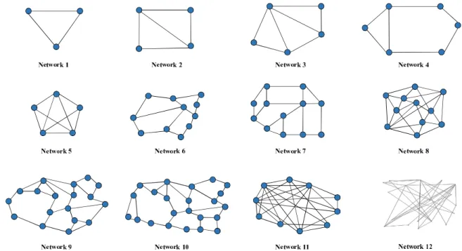
The simulation environment that we used are described as follows. In order to compare the results of MILP formulation and heuristic algorithm, four relatively small scale sample networks are used as shown in networks 1-4 of Figure 2.1. To determine the basic characteristics of the presented heuristic approach, eight sample networks are used as shown in networks 5-12 of Figure 2.1. Networks 5-11 mirror the typical backbone networks used to evaluate the routing performance in [61]. Network 12 is a random network generated using the BRITE topology generator [62] and the Waxman’s Probability model was used to create it. Table 2.1 summaries the basic characteristics of the sample networks in Figure 2.1. The link capacities of the sample networks were randomly generated with uniform
Figure 2.1: Sample networks used in the simulations
distribution in the range of (10Uc, 100Uc), where Uc[Gbit/s] is given a constant integer value. The maximum link weight, wmax, is set at 100. We confirmed that
wmax > 100 provides the same results as wmax = 100 in our examined networks.
Ic is set to 1000 after observing the trend of the worst-case congestion reduction of the presented scheme. The simulation program is coded in C language and executed on a Linux computer with 20GB of RAM. The linear programming problem in Equation (2.5) is solved using the IBM ILOG CPLEX Optimization Studio 12.4.
First, the performance of the presented heuristic approach is compared with the MILP formulation, which gives the optimal link weight set.
Let R denote the worst-case network congestion ratios of the sample networks 1-4 shown in Figure 2.1. The normalized worst-case network congestion ratio of the MILP is denoted as RM ILP and the normalized worst-case network congestion ratio of the presented heuristic approach is denoted as RP SO−C. The worst-case network congestion ratios are normalized using the results of MILP. The calcu-lated worst-case network congestion ratios are shown in Table 2.2 and following
2.5 Simulation results
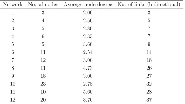
Table 2.1: Characteristics of the sample networks used to compare the heuristic and conventional schemes
Network No. of nodes Average node degree No. of links (bidirectional)
1 3 2.00 3 2 4 2.50 5 3 5 2.80 7 4 6 2.33 7 5 5 3.60 9 6 11 2.54 14 7 12 3.00 18 8 11 4.73 26 9 18 3.00 27 10 23 2.78 32 11 10 5.60 28 12 20 3.70 37
relationship is observed from the results.
RM ILP = RP SO−C (2.10)
This indicates that the link weight set calculated using the heuristic approach is able to provide similar performance as compared to the MILP for relatively small scale networks. This is related to the fact that the paths between node pairs in small scale networks are substantially fixed. Therefore, the path selected by both MILP and the heuristic are the same. Network 4 is the largest network we are able to solve due to computation complexity of the MILP formulation.
Then, the performance of the presented heuristic approach is compared with that of SO and RO via simulations. Network congestion ratio r is the performance measure of the evaluation.
The congestion ratio of SO without any link failure is used to normalize the calculated network congestion ratios of the sample networks. Let r(l) denote the network congestion ratio for link failure index l ∈ F . The normalized network
Table 2.2: Comparison of worst-case network congestion ratios of MILP and the heuristic Network RM ILP RP SO−C 1 1.00 1.00 2 1.00 1.00 3 1.00 1.00 4 1.00 1.00
congestion ratio of SO is denoted as rSO(l), the normalized congestion ratio of RO is denoted as rRO(l), and the normalized congestion ratio of the presented approach, P SO− C is denoted as rP SO−C(l).
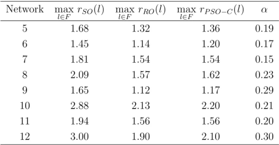
The worst-case network congestion ratios, max
l∈F rSO(l), maxl∈F rRO(l), and max
l∈F rP SO−C(l) of the sample networks 5-12 presented in Figure 2.1 for all single link failure scenarios are calculated as shown in Table 2.3. For the worst-case net-work congestion ratio for single link failure, the following relationship is observed.
max
l∈F rRO(l)≤ maxl∈F rP SO−C(l) ≤ maxl∈F rSO(l) (2.11) This indicates that the presented scheme is able to reduce the worst-case network congestion ratio as compared with SO. It also avoids the run-time link weight changes, which would cause network instability. As expected RO gives the optimal performance when a link failure occurs even though RO may lead to network instability. The achieved reduction rate of the worst-case congestion ratio, α, is defined as, α = max l∈F rSO(l)− maxl∈F rP SO−C(l) max l∈F rSO(l) . (2.12)
α is also shown in Table 2.3.
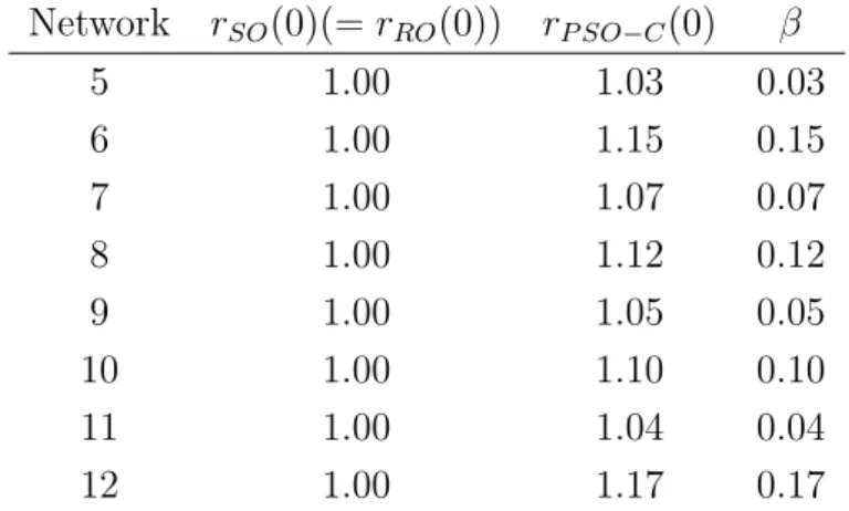
The normalized congestion ratios of no link failure are shown in Table 2.4. For the case of no link failure,
2.5 Simulation results
Table 2.3: Comparison of worst-case network congestion ratios of the heuristic and conventional schemes for single link failure scenarios
Network max l∈F rSO(l) maxl∈F rRO(l) maxl∈F rP SO−C(l) α 5 1.68 1.32 1.36 0.19 6 1.45 1.14 1.20 0.17 7 1.81 1.54 1.54 0.15 8 2.09 1.57 1.62 0.23 9 1.65 1.12 1.17 0.29 10 2.88 2.13 2.20 0.21 11 1.94 1.56 1.56 0.20 12 3.00 1.90 2.10 0.30
is observed. When there is no link failure, the congestion ratio of the link weight set obtained using PSO-C may be higher than that of SO or RO. This is because the objective of PSO-C is to reduce the worst-case network congestion ratio when link failure occurs. β is the deviation between rP SO−C(0) and rSO(0). β is defined as,
β = rP SO−C(0)− rSO(0) rSO(0)
. (2.14)
β is also shown in Table 2.4. When there is no link failure, β is the “penalty”
PSO-C has to “pay” to reduce the worst-case network congestion. The non-normalized simulation results show that the worst-case congestion ratios under single link failure is significantly larger compared to no link failure scenario.
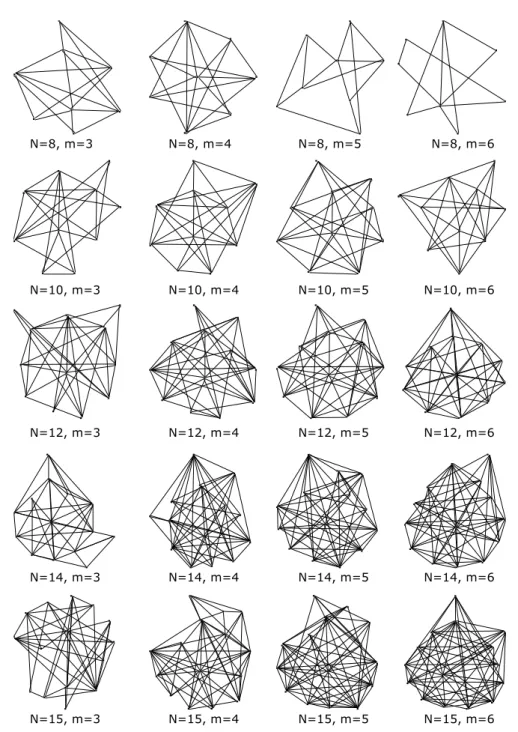
The worst-case congestion ratios of several random networks are calculated to understand the relationship between the worst-case congestion ratio and network topology. These random networks are generated using the BRITE [62] internet topology generator by changing the number of nodes N and the number of ad-jacency nodes m of the network. The Waxman’s probability model is used for interconnecting the nodes of the topology, which is given by,
P (u, v) = A exp(− d
Table 2.4: Comparison of network congestion ratios with no link failure Network rSO(0)(= rRO(0)) rP SO−C(0) β 5 1.00 1.03 0.03 6 1.00 1.15 0.15 7 1.00 1.07 0.07 8 1.00 1.12 0.12 9 1.00 1.05 0.05 10 1.00 1.10 0.10 11 1.00 1.04 0.04 12 1.00 1.17 0.17
where, 0 < A, B ≤ 1, d is the Euclidean distance from node u to node v, and L is the maximum distance between any two nodes. A and B are set to 0.15 and 0.2, respectively. The number of nodes, N , is set to 8, 10, 12, 14, 15 and the number of adjacency nodes m is set to 3, 4, 5, 6. The characteristics of the generated random network topologies are shown in Table 2.5 and the networks are shown in Figure 2.2.
The dependency of α on N and m is shown in Figure 2.3. This result shows that α is increasing with N for higher values of m (m = 5, 6). It means the dif-ference between the worst-case congestion ratios of SO and the presented scheme is increasing. This may relate to the increase in routing flexibility as N and m become higher. On the other hand, α fluctuates for smaller values of m. Smaller values of m or smaller number of neighbor nodes limits the selection of paths between source-destination pairs. This limited number of paths restricts the flex-ibility of the routing, causing α to fluctuate when links fail.
Figure 2.4 shows the dependency of β against N and m. Figure 2.4 indicates that the presented scheme is able to achieve the same result as SO for no link failure when the network becomes larger. This may occur because there is a wider number of routes to chose from when the network is larger.
In order to further show the effectiveness of the presented scheme, the worst-case congestion ratios of the presented scheme are compared with those of the two following link weight setting schemes. One is a scheme in which a link weight
2.5 Simulation results
Table 2.5: Characteristics of the random sample networks
N m Average node degree No. of links (bidirectional)
8 3 4.50 18 8 4 5.00 20 8 5 3.50 14 8 6 2.75 11 10 3 5.00 25 10 4 5.80 29 10 5 5.60 28 10 6 4.80 24 12 3 5.83 35 12 4 6.83 41 12 5 7.00 42 12 6 7.17 43 14 3 6.00 42 14 4 7.43 52 14 5 7.86 55 14 6 8.29 58 15 3 6.00 45 15 4 7.33 55 15 5 8.67 65 15 6 8.93 67
is inversely proportional to its capacity [31]. We call it the IPC scheme. The other scheme is the one in which all the link weights are set to one. As a result, minimum-hop routing is achieved. We call it the min-hop scheme. Table 2.6 shows the worst-case congestion ratios of the three schemes, which are normalized by that of the presented scheme. Table 2.6 indicates that the presented scheme reduces the worst-case congestion ratio, compared to the IPC scheme and the min-hop scheme. This is because the presented scheme determines link weights considering any single link failure so as to minimize the worst-case congestion ratio.
N=8, m=3 N=8, m=4 N=8, m=5 N=8, m=6
N=10, m=3 N=10, m=4 N=10, m=5 N=10, m=6
N=12, m=3 N=12, m=4 N=12, m=5 N=12, m=6
N=14, m=3 N=14, m=4 N=14, m=5 N=14, m=6
N=15, m=3 N=15, m=4 N=15, m=5 N=15, m=6
Figure 2.2: Random networks generated using BRITE
The allowable number of iterations to reduce the worst-case network conges-tion ratio is controlled by Ic. It is decided by considering the allowable computa-tion time, network size, and quality of the solucomputa-tion desired. A larger Ic increases
2.5 Simulation results
Figure 2.3: α’s dependency on number of nodes and adjacency nodes
the chance of getting a solution closer to the optimal one while the computation time increases. Our thorough examination on the effect of Ic suggests that the performance of the presented scheme remains unchanged after Icreaching an am-ple high value. Table 2.7 shows the effect of Ic for network 5, as shown in Figure 2.1. The results indicate that the performance of the presented scheme does not change after 1000 even if Icis increased. It suggests that, 1000 is large enough to converge the solution. We also confirmed the same tendency for other networks in Figure 2.1.
The results in Section 2.5 considers equal-cost multi-path (ECMP) [66] routing is employed. In non-ECMP routing networks, traffic is always routed over a single path, which often results in substantial network resources. On the other hand, ECMP routing distributes the traffic among several equal cost paths instead of routing all the traffic along a single best path. Fundamentally, ECMP routing can be more efficient compared to single path routing protocols because it can reduce
Figure 2.4: β’s dependency on number of nodes and adjacency nodes
congestion in “hot-spots”, by deviating traffic to unused network resources, thus providing load balancing.
In order to confirm the effectiveness of ECMP routing, the worst-case con-gestion ratios of ECMP routing are compared with that of single path routing for sample networks 5-12 shown in Figure 2.1. Table 2.8 summarizes the worst-case congestion ratios of ECMP routing and single path routing. The worst-worst-case congestion ratios of ECMP routing is expressed as rP SO−ECMP while rP SO−single expresses the worst-case congestion ratios of single path routing. The worst-case congestion ratios in Table 2.8 are normalized by rP SO−ECMP.
ECMP routing’s ability to distribute the traffic among several equal cost paths is confirmed from Table 2.8. It is observed that the difference between ECMP routing and single path routing increases with average node degree. Higher av-erage node degree increases the number of paths between nodes, thus raising the possibility of multiple equal cost paths in the network. As a result, ECMP
rout-2.5 Simulation results
Table 2.6: Comparison of worst-case congestion ratios with different link weight setting schemes
Network Presented scheme IPC scheme min-hop scheme
5 1.00 1.82 2.05 6 1.00 2.45 2.76 7 1.00 3.16 3.74 8 1.00 2.35 2.69 9 1.00 1.83 2.21 10 1.00 3.42 3.52 11 1.00 2.70 2.72 12 1.00 1.58 2.19
Table 2.7: Comparison of presented scheme’s performance related to Ic
Value of Ic Worst-case congestion 100 0.553 200 0.411 300 0.403 400 0.403 500 0.359 600 0.260 700 0.224 800 0.183 900 0.183 1000 0.183 1200 0.183 1500 0.183
ing is able to distribute traffic among these multiple equal cost paths and reduce the congestion.
Table 2.8: Comparison of worst-case congestion ratios of ECMP routing and single path routing
Network Average node degree rP SO−ECMP rP SO−single
5 3.60 1.00 1.02 6 2.54 1.00 1.02 7 3.00 1.00 1.03 8 4.73 1.00 1.08 9 3.00 1.00 1.02 10 2.78 1.00 1.02 11 5.60 1.00 1.08 12 3.70 1.00 1.04
Chapter 3
Path selection scheme for energy
consumption reduction with link
failure and traffic uncertainty
3.1
Energy saving routing
How to reduce the energy consumption has recently become a major concern for industries due to economic and environmental reasons. The core network equipments currently occupy 20% of the total energy consumption and it is not showing any sign of slowing down [63]. Therefore, saving energy has also become one of the objectives of network service providers.
In present high speed networks, the link capacities of backbone networks are often over-provisioned in order to permit re-routing when links fail. If the back-bone network is already optimized considering link failures, it is possible to reduce the network energy consumption by switching off unused resources or putting them into sleep mode. In today’s backbone networks, pairs of nodes are typi-cally connected by multiple physical cables to accommodate more traffic or for future extension purposes. These links are usually over-provisioned only con-sidering network reliability reducing network energy efficiency. Previous studies [64, 65] show that less than 40% of network link capacity is utilized on average, suggesting 60% of the energy consumed by links are wasted on average. Accord-ingly, shutting down individual unused bundled cables can achieve energy saving