Hands-free Speech Recognition by a microphone array and HMM composition
6
0
0
全文
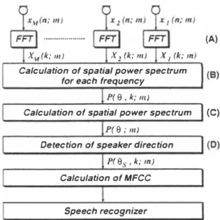
(2) Sp制kør localizer. (A). 1x. x",{k;川). 2. 1X. (k;・川. I. (伏k;川. 1 (8町). Calculation ofs叩pati,ωalゆpowerspect叩m fOr each frequency P(S.k;lII). Figure. 1:. I (C). Calculation ofspatial powerspectrum. Block diagram of the SLAM system. P{S; 111). 1(0). Detection ofspeaker direction processing.. P(Ss' k; m). It is assumed that a plane wave. Calculation of MFCC. comes from the direction () to the equally spaced array composed of lvf microphones,. Speech recognizer. where the plane wave is a complex sinusoidal signal in frequency. f,. and d denotes the dis. tance between two adjacent microphones. The. Figure 2: Algorithm of the SLAM system. Xl(t),・・・, XM(t). ) 1ム (. outputs of each microphone are given as follows:. η,. 民(t)=Xl(tー(i-1) 学). i. is micro. m. are sample index, frequency index,. In order to estimate sound source directions. ()lγ・.. ()r, the spatial power spectrum which. ,. defined by Eq. (3 ) is calculated.. and-sum beam-former is given as follows:. where. P. (() k; ,. m. ). m. P. m. P. 2 州+(i-1)午�) = 2 2zw(mt-l)与午). Mt) =. (2),. and. (B) (C) Sound source direction estimator. Then the output of the delay. As a result of Eq.. k,. and frame index, respectively.. 守d nu nRu nu -no 'K ハσ ね 乞 同 一一 nσ. where c is the sound velocity and phone index.. ,. is equivalent to the output. power of the delay-and-sum beamformer, and is given as follows:. a signal comes from the. direction B is M times as large, while signals. = l bz(丸山p {j27rfk(i-l)�引 い () = 0,1,・・・,180 fk. come from different directions aren't enhanced. Therefore the directivity which is sensitive to the direction B is formed.. 2.2. SPEAKER. LOCALIZATION. ALGORITHM. responding frequency to. k. r. (A)(B)(C)(D). of directions on the spatial power spectrum.. (0) Speaker direction detector. in Fig.2. are described as follows.. A. (A) Frequency analyzer. In order to ap. speaker. direction. Bs. is. (B)(C).. in. band. power spectrum is obtained as. the. outputs. of. each. micro. phone are divided into K frequency compo. 0,・・・,. (η;m),・・" XM(η;m) Xdl.:;m)γ・・, .\1'v[(1.:; m). based. nents. In Fig. 2, Xl. and. denote the outputs of. each microphone and the FFT of them. Where. from. K. -. As a result, a enhanced speech. P B s , k;. (. m), 1.: =. 1.. I A simple speaker localization algorithm is on. extracting. (SLAM司P). SLAM-P. 1150 44. detected. among the sound source directions estimated. ply the delay-and-sum beam-former for broad signals,. sound source di. rections are obtained by detecting every peaks. An algorithm of the SLAM system is shown in Fig. 2. The details of. denotes a cor. and. where. the. maximum. power. is represented as Bs. =.
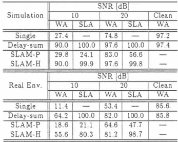
(3) argmaxe P(8..,; m) , where 8.., denotes one of r 、 sound source directions. However this algo. Fig.4. The gain for 40 degree in computer sim 一一in comput.r simul.t;on. ーー n i. rit.hm wiU be in trouble in low SNR conditions.. ,..1 .nvironm・nt.. Sρ・.1<,・r dJr・ction. In this papぞれa speaker localization algorithm. .... based on extractillg a pitch harmonics (SLAM H) is used to localize a speaker direction accu. f. rately in low SNR conditions. SLAM-H is rep. P(8s; m ) , where 88 ó denotes one ofムsound source directions ex. /. resented as 85 = argmaxo. tracted a pitch harmonics.. -'0. 。. ,j15-Notse soum ,J1 \\_ � 殴 ニ.- Jì.V73 (.it Y ・4,r ! .ction. ・20. ・20. -'0. 。. aain (d8AJ. Ifム= 0, then a. speaker direction which detected previously is. Figure 4: Directivitional Pattern. used for current frame.. ulation and real environments are. 2.3. EXPERI加lENTS. and. The microphone array is a equaUy spaced ar ray composed of 14 microphones, where the. 2.4. distance between two adjacent microphones is. -17.3. dB.. -21.7. dB. RECOGNITION RESULTS. The word recognition accuracy (羽rA) and. 2.83 cm. The speaker direction and the . Gaus・. speaker localization accuracy (SLA) are shown. sian noise source direction are at 90 degree and. in Table 1.. 40 degree.. Delay-sum is the case that a. The outputs of each microphone Word Recognition Accuracy and. are generated considering only the time differ. Table 1:. ences. In real environments, the experimental. Source Localization Accuracy. room as shown in Fig.3 is used for recording.. SNR [dB]. The reverberant time in this room is about 0.18. Simulation. 5.83m. WA Single Delay-sum SLAM-P SLAM-H. 弘 ・hM 旬 、コ. e k P S . ji llr. SLA. Clean WA 97.2. 90.0. 100.0. 97.6. 100.。. 29.8. 24.1. 83.0. 56.6. 90.0. 99.9. 97.6. 99.8. Single Delay-sum SLAM-P SLAM-H. speaker and a Gaussian noise source. The recognition algorithm is based on 256 Tied Mixture HMM. Speech signals are sam pled at 12 kHz and windowed by the 32 ms Hamming window every 8 ms, and then calcu lated 16・order MFCCs and 16・order 6 MFCCs The recognition experiment. is conducted for speaker dependent 500 words To evaluate the performance of. the SLAM system, Word recognition Accu racy (WA) and Speaker Localization Accuracy (SLA) are used.(within土30) The directional pattern obtained for 6 kHz band-limited Gaussian noise in computer sim ulation and real t'nvironments are ShOWll in. 20. 10. WA. Two loud speakers are substituted for a. recognition.. WA 74.8. 27.4. Real Env.. Figure 3: Experimental Room. and aムPower.. 20. SLA. 9ï.4. SNR [dB]. と� �ω1m. sec.. 10. SLA. 11.4. WA. SLA. Clean WA 85.6,. 53.4. 64.2. 100.0. 82.0. 100.0. 18.6. 21.1. 64.6. 47.7. 55.6. 80.3. 81.2. 98.7. 85.8. speaker direction is known. Th.is should be an upper bound of the performance of the SLAM system.. On the other hand, SLAM-P and. SLAM・H are the speaker direction unknown condition.. Clean is the case that a Gaussian. noise source isn't located (SNR 38 dB). This table confirms that the SLAM system with ex traction of pitch harmonics attains the much higher speech recognition performance than that 01' a single microphone not only in com puter simulation but also in real environments. Thére still remains degradation in the real en vironment. The de-reverberation of acoustical transfer function and normalization of micro phone elements will be llecessary. 1151. 45.
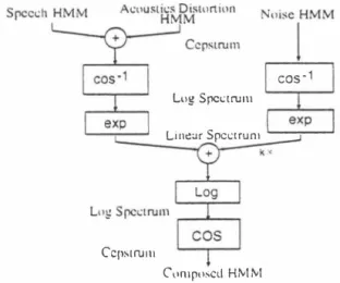
(4) 3. HMM COMPOSITION. nal. respectively.. In this sedion HMM composition method for. additive noisぞ. is introduced.. and room reverberation. �'lany works are presellted. to solve noise alld. reverberation problems. served in linear spectral domain, we regard O(t), S(t), N(t) as short time linear spectra whose analysis window starts at time t from now on. Gell引'ally , parameters for speech recognition. from the points of speech enhancemellt and model modification.. As for the speech en. Since this relatioll is pre. are represented by the cepstrum.. The pa. the spectral subtrac. rameters have to be transformed to linear do. tion method for an additive noise and the. main as an addition of the speech and noise. cepstral mean normalization method. holds[10, 12].. hancemellt approach,. for a. As for a convolutional distortion, the ob. cOllvolutional noise had been proposed and confirmed their effectiveness[1,. 9].. As for. served distorted spectrum is represented by. the model modification approach, the con. 。(t) = H(t)・S(t). ventional multi-template approach, and model adaptation approach[13] and the model (de・ )composition approach[2, 10, 12] had been pro Amoug these approaches the HMM. posed.. composition approach is promising, because the HMM for the noisy speech can be eぉ ily generated by composing the speech HMMs. where H(t) is a transfer function from the sound source to the microphone.. H(t) is a. function of time t since the sound source may move. The multiplication can be converted to sum in cepstral domain as,. and the noise HMM which trained during noise period.. 。cep(t) = Hcep( t) + Scep(t). The papers[10, 12] shows the com. posed noisy HMM outperforms very high ac curacy.. The papers[ll, 14] also try to apply. the method to telephone channel adaptation. In this paper, we apply the HMM composition to the recognition of the speech which is con. where, O cep(t), Hcep(t) and Scep(t) are cep stra for the observed signal, acoustic trans fer function and speech signal, respectively. Therefore the observed signal is represented b y. taminated by not only an additive noise but also the room reverberation[15]. 3.1. 。(t) = e xp( F( 5 cep(t) + Hcep(t)) ) + k N(t) (5 ). THEORY. On the assumption that the speech and noise signal are independent, the observed signal is. 恥伽Spcc<.:hαωωじd山h一1. represented by. 。(t) = S(t) + N(t). Lllg S pc<.: t ru 111. The conveutional approach estimates noise. Lin白r Spc<.:trum. statistics during the noise period and recog. I c。凶'S-1 -------r-一 I. exp. I. �一一一ー. nizes an input noisy speech by using the noise added reference patterns. The HMM composi・ tion executes addition in HMM parameter do main instead of the addition in signal domain. Since the signal level is generally different be tween training and testing, an adjustment fac tor k is introduced. Thus the observed signal is represented by. 。(t). C川lIpuscd HMM Figure .): Block diagram of HMM Composition This procedure is summarized in Fig.5. The. =. O(t)、S(t). çosille transform. inverse cosine transform, ex. S(t) +んN(t) N(t). ponential transform and log transform are con・. are the observed. ducted 01\ HMM parameters. The HMM rec・. lloisy signal, speech sigllal and lloise sig-. つgnizer decocles the observed sigllal 011 a trellis. where. 46. CCflstrulll. and. 1 152.
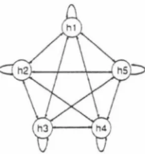
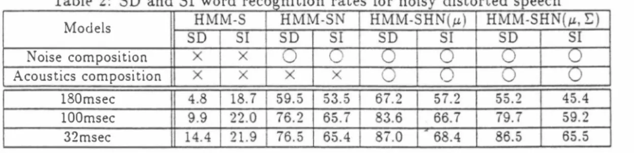
(5) diagram according to max.iITÙze the log like lihood.. Decoded path will bring a optimal. combination of a speech, transfer function and nOlse.. 3.2. EXPERI乱1ENTS. The recogllitioll experiments are conducted for degraded speech uttered in a same room used in section 2. Fig.6 shows the room used in the experiment. We measured 9 transfer func tions from 9 positions to the ITÙcrophone. The former five positions, h1,・・・,hs are used for. Figure í: Ergodic HMM of acoustical transfer function. the model composition and the latter four po・ sitions, Pl, ・・,P4 are used for the recognition tests. The transfer functions are measured by the sweep method. The test data are simulated by the linear convolution of speech corpus and the measured transfer function.. wiU be atfected by the predecessor samples, HMM would be able to model the variation by covariance matrix, E, of Gaussian pdf. The results are listed in Table.2. The results clar ify the effectiveness of the proposed method for noisy and reverberant speech recognition. The. hllJ Pl[J. etfect of a length of the impulse response is also exaITÙlled. The several distorted signals are ar . ヨ. tificially made by L=180,100 and 32msec im. p2 [J. pulse respOIlses by adjusting the original one.. h21J. The Table. 2 also shows those results by HMM composltlOn. Next, we evaluate the performance of the model for the unknown testing sound source. Figure 6: Room environment. positions. Table.3 shows average SD recogni. Speech corpus and analysis conditions are. tion rates for the known training and unknown. the same as section 2. Speaker dependent(SD). testing positions in 180msec reverberation. It. and independent(S1) HMMs are prepared. The. is confirmed that the degradation between the. S1 HMMs are trained by 64 speakers. The 500. training and testing sound source positions is. words both in training data set and testing. relatively small for all composed HMM.. data set are used for recognition evaluation.. 4. The experiments are carried out by using two. CONCLUSION. male and two female speakers. The noise data. This paper describes two novel approaches to. is collected in a computer room and added to. solve the problems of robust speech recogni. the clean speech data or acoustically distorted. tion ill noisy reverberant room.. data as the SNR is 15dB. Firstly, the. approach based on SLAM, the speaker 10-. We assigned one state for the noise HMM. calization by using arrayed llÙcrophones, is. and 5 states for the HMM of the acoustical. presented.. The experiments show that the. Fig. ï shows the structure. delay-and-sum beam-former improves SNR by. of the HMM of the acoustical transfer func. +20dB in 500 and the proposed localization. tion. Each state direct.ly corresponds to one of. algorithm estimates the speech source direc. the t.raining positions, h1,・・・, hs・ The single. tiOll accurately. SLAM-H achieves the recog・. Gaussian p df is llserl for these HMMs.. nition rates close to those of speaker direction. transfer functioIl.. The t.ransfer function in cepstral domain is. kno、�n case. Secondly, the HMM composition. obtained by subtracting the cepstrum coeffi. approach with a single microphone for an ad. cients of original speech from those of cOllvolu. clitive noise and room acoustical distortion is. tioned spt>ech. However this transfer function. presented.. The performance is evaluated by. 1153. 47.
(6) Models Noise composition Acoustics composition 180msec 100msec 32msec Table. 3:. Results for known and unknown positions (L=180msec ). Models Acoustics composition. I. I. HMM-S. HMM-SH(μ). I. HMM-SH(μ,E). Distorted speech the noisy and reverberant speech. The results show that the proposed HMM composition im proves the recognition accuracy from 4.8% to 67.2% for SD test by the HMM composition. These two approaches are quite effective to realize hands-free speech recognition in real adverse environments.. Furthermore comple. mentary combination of these approaches will bring more effective hands-free speech recogni tion system.. References [1] S.F.Boll,喝uppression of acoustic noise in speech using spectral subtraction", IEEE Trans. ASSP・2ï, 4, pp. 113-120, April 19ï9. [2] A.P.Varga,R.K.Moore,“Hidden Markov Model Decomposition of Speech and Noise", ICASSP90, SI5b.l0, pp. 845-848, April 1990. [3] J.L.Flanagan, R.Mammone, G.W.Elko, “Au t凶。dωlr閃ective mi比crophon号 syst怜em for natural communication with speech rec∞ogmz白er凶s DARP臥A Workshop on Speech and Natural Lan guage, pp.4.8・4.13, 1991.2 [4] H.F.Silverman, S.E.Kirtman, J.E.Adcock, P.C.Meuse, "Exper imental results for baseline speech recognition performance using input acquired from a lin ear microphone array", 5th DARPA Workshop on Speech and Natural Language, pp.285・290, 1992 [5] D.Van Compernolle, W.Ma, F.Xie, M.Van Di est,“Speech recognition in noisy environments with the aid of microphone arrays",Speech Communication‘9(5/6) pp.433・442, 1990 [6] Q.Lin. E.E.Jan‘C.Che, B.de Vries, '‘System of microphone arrays and neural networks for ro・ bust speech recognition in multimedia environ-. ment", ICSLP94, S22・2, pp. 124ï-1250, Sep. 1994. [ï] D.Giuliani, M.Matassoni, M.Omologo, P.Svaizer,“Hands-free continuous speech recognition in noisy environment using a four microphone array", ICASSP95, pp.860・ 863, 1995 [8叫] T.Yamada払, S.N、J匂九ωJ匂raω.k伶町atrロm speech recogni比tlωon with speaker localization by a microphone arロrayγ",ICSLP96 1996,10 [9] A.Ace 叫 Acoωtical and enviroπm刊tal robust πess in automatic speech recognitioπ. Ph.D Dis sertation, ECE Department, CMU, Sept.1990 [10] M.J.F.Gales, S.J.Young, “An improved ap proach to the hidden Markov model decompo sition of Speech and Noise",ICASSP92, pp.233・ 236, 1992 [11] M.J.F.Gales, S.J.Young, “PMC for speech recognition in additive and convolutional noise", CUED-F・INFENG-TRI54, 12, 1993 [12] F.Martin, K.Shikano, Y.Minami, "Recogni・ tion of noisy speech by composition of hidden Markov models", EUROSPEECH93, pp.1031・ 1034, 1993 [13] A.Sa此ar, C-H.Lee,“Robust speech附ogni・ tion based on stochastic matching", ICASSP95, pp.121・124, 1995 [14] Y .Minami,S.Furui, "A maximum likelihood procedure for a universal adaptation method based on HMM composition", ICASSP95, pp.129・132, 1995 [15] S.Nakamu民T.Takiguchi, K.Shikano,“Noise and acoustics distorted speech recognition by HMM composition", ICASSP96, pp.69・72, 1996. 1154 48.
(7)
図
+2
関連したドキュメント
6 Scene segmentation results by automatic speech recognition (Comparison of ICA and TF-IDF). 認できた. TF-IDF を用いて DP
Found in the diatomite of Tochibori Nigata, Ureshino Saga, Hirazawa Miyagi, Kanou and Ooike Nagano, and in the mudstone of NakamuraIrizawa Yamanashi, Kawabe Nagano.. cal with
In order to estimate the noise spectrum quickly and accurately, a detection method for a speech-absent frame and a speech-present frame by using a voice activity detector (VAD)
patient with apraxia of speech -A preliminary case report-, Annual Bulletin, RILP, Univ.. J.: Apraxia of speech in patients with Broca's aphasia ; A
Recently, Arino and Pituk [1] considered a very general equation with finite delay along the same lines, asking only a type of global Lipschitz condition, and used fixed point theory
のようにすべきだと考えていますか。 やっと開通します。長野、太田地区方面
Although the choice of the state spaces is free in principle, some restrictions appear in Riemann geometry: Because Einstein‘s field equations contain the second derivatives of the
ShiraZucker TheBlack-and-WhiteColoringProblemonChordalGraphs JournalofGraphAlgorithmsandApplications
In general, the algorithm takes a chordal graph G, computes its clique tree T and finds in T the list of all non-dominated pairs (b, w) such that G admits a BWC with b black and w
