Voronoi図を用いた多次元データの補間 (新しいパラダイムとしてのアルゴリズム工学)

Voronoi

$\backslash d$

を用いた多次元

$\overline{7}^{--}\backslash \backslash$

タの補間

Interpolation of Multivariate

Data

Using Voronoi Diagrams

日吉久礎1 杉原厚吉2

HisamotoHIYOSHI $\mathrm{K}\mathrm{o}\mathrm{k}\mathrm{i}\mathrm{c}\mathrm{l}\dot{\mathrm{u}}$

SUGIHARA

東京大学大学院工学系研究科

〒 113-8656_{東京都文京区本郷}7-3-1

[email protected]

$z_{\mathrm{S}\mathrm{u}\mathrm{g}\mathrm{s}}\mathrm{i}\mathrm{h}\mathrm{a}\mathrm{r}\mathrm{a}@\mathrm{i}\mathrm{m}\mathrm{P}^{1\mathrm{t}\mathrm{O}}\mathrm{e}\mathrm{x}.\mathrm{t}.\mathrm{u}-\mathrm{k}\mathrm{y}\mathrm{o}.\mathrm{a}\mathrm{C}$ ip

Abstract: This paper presents a general framework for constructing a variety of

multi-dimensional interpolants based on Voronoi diagrams. This fr\v{c}unework includes previously

known methods such as Sibson’s interpolant and Minkowski’s interpolant;

moreover

it

con-tainsinfinitelymanynewinterpolants. Computational experiments suggest that the

smooth-nessimproves by theproposed generalization. Hence. this framework gives a newand

promis-ingdirection of researcll on the interpolation based on the Voronoidiagrams.

Keywords: Voronoi diagram, multivariate data interpolation. spatial surface.

1

Introduction

Interpolation is an extremely important

tech-nique to solve various problems in engineering

suchas differential equations and geometric

mod-cling. The finite element method is one of the

most practical approaches to the interpolation

problem, and is well-established today. However,

there is an alternative approach to the

interpo-lation problem, which utilizes Voronoi diagrams.

In this paper, we call this approach the Voronoi

diagram approach. See, for example, [1, 5, 6] for

the theory of the Voronoi diagrams.

Theinterpolation problem is formulated in the

following way. Let $\varphi$ :

$\mathrm{R}^{d}arrow \mathrm{R}$ be a function,

whose value is known onlyon the points $P_{1},$

$\ldots$ ,

$P_{n}$

.

These points are called the data sites. The

(exact) interpolation problem is to find a good

function $\tilde{\varphi}$ such that

$\tilde{\varphi}(P_{i})=\varphi(P_{i})$

for$\dot{i}=1,$

$\ldots,$$n$. The meaning of the word “good”

dependson the context.

Thiessen first applied Voronoi diagrams to the

interpolation problem [11]. Let $P$ be the target

point the valueon whichisto beestimated. In his

method, theVoronoidiaglam for the data sites is

constructed. Assume that the point $P$ bclongs

to the Voronoi region of $P_{i}$

.

Then, the value at

$P$ is estimated at the value at the point $P_{i}$

.

By

the definition, Thiessen’s interpolant is a

picce-wise constant function.

Recently, Sibson found anotller intcrpolation

method $[8, 9]$

.

In his method, the Voronoi

dia-gram for $\{P_{1,}\ldots.’.P_{n}, P\}$ is constructed. If the

Voronoi regions of $P$ and $P_{i}$ arc adjacent via a

$(d-1)$-dimensionalfacet, wecall$P_{i}$ aneighbor of

$P$. The critical fact he found is that the position

vector of $P$ can be expressed as a convex

com-bination of the position vectors of$P’ \mathrm{s}$ neighbors

with the coefficients computed from the

second-order Voronoi diagram [8]. Hence we can

inter-pret the coefficients of this convex combination

as

the coordillates of $P$. Sibson constructcd $\mathrm{C}^{0}$

and$\mathrm{C}^{1}$ interpolants basedonthis coordinate

sys-tem. Sibson’s interpolation method

was

further

pro-posed another $\mathrm{C}^{1}$

interpolant $\mathrm{b}\mathrm{a}s$ed

on

the

Bern-stein polynomial [2].

On the other hands, Hiyoshi and Sugihara

found another coordinate system, and proposed a $\mathrm{C}^{0}$

interpolant [3, 4, 10]. We call this

sys-tem Minkowski’s coordinate syssys-tem, because it

is based on the Minkowski’s theorem on convex

polytopes.

Compared with the finite element

interpola-tion, the Voronoi diagram approach has a lot

of virtues [9]. For example, interpolants based

on the Voronoi diagram approach behaves

con-tinuously when the data sites move. However,

the Voronoi diagram approach is less flexible in

some points: for example, it is difficult to

con-struct even $\mathrm{C}^{2}$

interpolants by tlle Voronoi

dia-gram approach, as explained in Section 2. The

main reason, we guess, is that the number of

the coordinatesystems that thc Voronoi diagram

approach stands on is too few. In this paper,

we generalize the coordinate systems in order to

make the Voronoi diagram approach more

flexi-ble,concentratingonthecasewhen$d=2$

.

$\mathrm{I}\mathrm{n}\mathrm{d}$

.eed

we construct a large class of interpolants based

on the Voronoi diagram approach, which

con-tains both Sibson’ and Minkowski’s interpolants,

and which contains infinitely many other

inter-polants. Computationalexperimentssuggest that

the smoothness improves by the proposed

gener-alization. Hence, this generalizationgives a new

and promising direction ofresearch on the

inter-polationbased on the Voronoi diagrams.

Section 2 reviews Sibson’s coordinate system

and Minkowski’s coordinate system. Section 3

gives another proofto Sibson’sresult, which

pro-vides the basic idea of

our

generalization.

Sec-tion4 proposes the generalization. Section5 gives

some

computational experiments. Section 6

con-cludes

our

research.

2

Previous Works

In this section, we review the previous works

briefly.

2.1

Notations

First, let us introduce some notations.

Assume that a finite number of points $P_{1},$

$\ldots$ , $P_{n}\in \mathrm{R}^{2}$ aregiven. $P_{i^{\mathrm{S}}}$’ arecalled the generators.

Let $V(P_{i})$ be the set of all the points $Q\in \mathrm{R}^{2}$

such that $\mathrm{d}(Q, P_{i})<\mathrm{d}(Q_{B}.P_{j})$ for $j\neq\dot{i}$, where

$d(P, Q)$ _{denotes the Euclidean distance between}

two points $P$ and $Q$

.

We

call

$V(P_{i})$ the Voronoi

region of the generator $P_{i}$

.

By the definition,

the boundary of eacll $V(P_{i})$ is a convex polygon.

The Euclideanplane$\mathrm{R}^{2}$is almostpartitionedinto

$V(P_{1})’\ldots$

.

$,$

$V(P_{lt})$, that $\mathrm{i}\mathrm{S},\cdot$ the

measure

of the set

of all the point that does not belong to any $V(P_{i})$

is

zero.

The collection of all $V(P_{i})’ \mathrm{s}$ is denoted

by $\mathcal{V}(P_{1}, \ldots’.P_{n})$ and is called the Voronoi $d\dot{i}a-$

gram for the generator set $\{P_{1,}\ldots. , P_{n}\}$. When

two Voronoi regions$V(P_{i})$ and$V(P_{j})$

are

adjacent

via some open line segment, this line segment is

called the Voronoi

_ed.

$qe$ between $P_{i}$ and $P_{j}$, and

is denoted by $E(P_{i}, P_{j})$

.

If$E\langle P_{i},$ $P_{j}$) exists, $P_{j}$ is

called a neighbor of$P_{i}$ (and vice versa).

For $i\neq j$, let $V(P_{i}, P_{j})$ be the set of all the

points $Q\in \mathrm{R}^{2}$ such that

$\mathrm{d}(Q\text{ノ}.P_{i})<\mathrm{d}(Q, P_{j})<\mathrm{d}(Q, P_{k})$

for $k\neq i,j$

.

$V(P_{i}, P_{j})$ is called the second-order

Voronoi region of the ordered pair $(P_{i}, P_{j})$

.

By

the definition, each $V(P_{i})$ is almost partitioned

into $V(P_{i}, P_{j}),$ $i\neq j$

.

The collection of all

$V(P_{i}, P_{j})\prime \mathrm{s}$ is called the second-order Voronoi

di-agram for the generator set $\{P_{1}, \ldots, P_{n}\}$.

See, for example, [1, 5,6] for the detail of the

Voronoi diagram theory.

2.2

Sibson coordinates

Now let us describe Sibson’s interpolation

method $[8,9]$ briefly.

Let $P_{1},$

$\ldots$

,

$P_{n}\in \mathrm{R}^{2}$ be the given data sites,

and let $y_{1},$ $\ldots$

,

$y_{n}\in \mathrm{R}$ be the data value

associ-ated with $P_{1},$

$\ldots,$ $P_{n}$, respectively. Assume that.

we walltto evaluate the valueonthe target point

It follows from the definition that

Figure 1. The $\mathrm{V}\mathrm{o}\mathrm{l}\cdot \mathrm{o}\mathrm{n}\mathrm{o}\mathrm{i}$ region $V(P)$ is

parti-tioned into $\mathrm{t}\mathrm{l}$

)$\mathrm{e}$ subregions $V(P, P_{i})$.

the

convex

hull of$P_{1\cdot*},$

.

, $P_{n}$, but does not equal

to any of$P_{1_{B}}.\ldots,$ $P_{n}$

.

According to Sibson [8], the Voronoi diagram

$\mathcal{V}(P_{1}\ldots..P_{l},, P)$ is constructed. Each $V(P_{i})$ is

not necessarily bounded, but $V(P)$ is always

bounded because $P$ is an ipner point of the

con-vex hull of $P_{1_{\mathrm{P}}}.\ldots$ , $P_{1},$

.

Now partition $V(P\rangle$ into $V(P, P_{i})\mathrm{s}$, and let $s_{i}^{1}(P)$ denote the

measure

of

$V(P, P_{i})$

.

Note that $s_{i}^{1}(P)>0$ if and only if$P_{i}$ is

a neighbor of$P$.

Figure1 shows this situation. Inthisfigure, the

Voronoiregion$V(P)$ is partitioned into the

subre-gions $V(P, P_{i})$. The boundaries of this paltition

are drawn by the dashed lines.

Let $x_{1},$ $\ldots$

,

$x_{r\iota}$ and $x$ denote the position

vec-tors of$P_{1},$

$\ldots$

,

$P_{tl}$ and$P$, respectively. Sibson [8]

proved the following identity:

$\sum_{i=1}^{n}s_{i}(1P)x=\sum_{i=1}^{n}s^{1}i(P)\%$. (1)

We will give another proof of thisidentity in

Sec-tion $3\text{ノ}$

.

which gives the basic idea of the

general-ization we propose. Now define that

$\hat{s}_{i}^{1}(P\rangle=s^{1}i(P)/\sum^{n}s_{j}(1P)j=1^{\cdot}$

$\sum_{i=1}^{n}\hat{S}i(1P)=1$, $0\leq\hat{s}_{i}^{1}(P)\leq 1$

.

Thus $x$ is expressedas the following

convex

com-bination:

$x= \sum_{i=1}\hat{S}_{i(}^{1}P)x_{\iota}n$.

We call$\hat{s}_{i}^{1}(P)\mathrm{i}\mathrm{s}$thc Sibson coordinates of the point $P^{1}$

.

Note that $\hat{s}_{j}(P)arrow\delta_{ij}$ as $P$ approaches $P_{i}$.

Therefore we dcfine

$\hat{s}_{7}^{1}(P)=\delta_{i;}$

wllen $P$ coincideswith $P_{i}$

.

From the Sibson coordinates, Sibson

con-structed the following $\mathrm{C}^{0}$ interpolant:

$\tilde{\varphi}^{1}(P)=\sum_{i=1}^{n}yi\hat{S}^{1}i(P)$

.

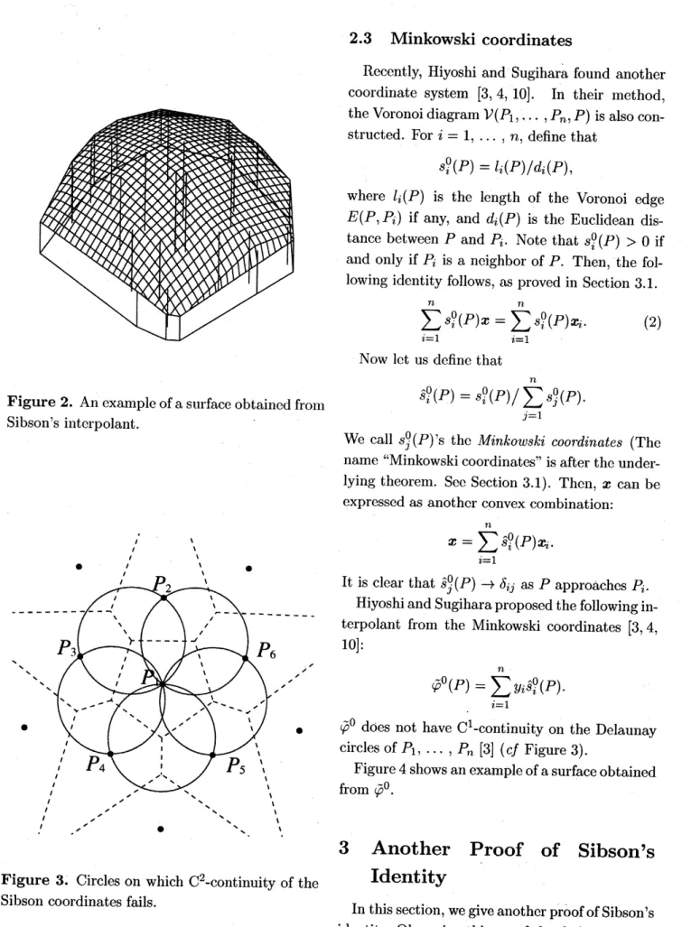
Figure 2 shows an example ofa surface obtained

from the aboveinterpolant.

Although $\mathrm{C}^{1}$ interpolants has been also

pro-posed by Sibson [9] and Farin [2], it is difficult

to construct interpolants that have higher-order

continuity. This difficulty

comes

from a global

property of $\hat{s}_{i}^{1}$. Piper showed that $\hat{s}_{i}^{1}\mathrm{s}$

are

dif-ferentiable everywhere except the points $P_{i\mathrm{p}}$. but

$\mathrm{C}^{2}$-continuity fails on the Delaunay circles of the

data sites [7]. Devising a technique to avoid this

non-smoothness is difficult.

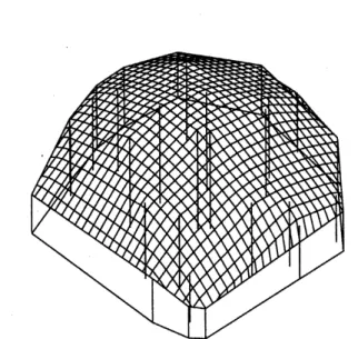
Figure 3 shows where $\mathrm{C}^{2}$-continuity fails. In

this figure, the Voronoi diagram for the 11 data

sites is drawn by dashed lines. In particular, the

generator $P_{1}$ has five neighbors $P_{2},$ $\ldots$ , $P_{6}$. In

other words, the boundary of the Voronoi region

of$P_{1}$ is a pentagon. Hence, there

are

five

Delau-nay circles that

are

concernedwith $P_{1}$, on which

the $\mathrm{C}^{2}$-continuity of$\hat{s}_{1}^{1}$

.

1wealso call$s_{i}^{1}(P)’ \mathrm{s}$ the Sibson coordinates when there

is llo collfusion. Isfact, $(s_{1}^{1}, \ldots , s_{n}^{1})$ and $(\hat{s}_{1}^{1}, \ldots,\hat{s}_{n}^{1})$

de-note thesamepointin the$(n-1)$-dimensionalreal projec-tive space.

2.3

_{Minkowski coordinates}

Figure 2. Anexampleofasurface obtained from

$\mathrm{S}\mathrm{i}\mathrm{b}\mathrm{S}\mathrm{o}\mathrm{n}\mathrm{s}$ interpolant.

Recently, Hiyoshi and Sugihara found another

coordinate system [3, 4, 10]. In their method,

theVoronoi diagram$\mathcal{V}(P_{1}, \ldots’.P_{n,}.P)$ isalso

con-structed. For $\dot{i}=1,$ $\ldots \mathrm{l}n$, define that

$s_{i}^{0}(P)=l_{i}(P)/di(P)$,

where $l_{i}(P)$ is the $1\mathrm{C}\mathrm{n}\mathrm{g}\mathrm{t}1_{1}$ of the Voronoi edge

$E(P, P_{i})$ if any, and $d_{i}(P)$ is the Euclidean

dis-tance between $P$ and $P_{i}$

.

Note that _{$s_{i}^{0}(P)>0$} if

and only if$P_{i}$ is a neighbor of$P$

.

Then, the

fol-lowing identity follows,

as

proved in Section 3.1.

$\sum_{i=1}^{n}s_{i}(P0)X=\sum_{i=1}^{n}S_{i}(0P)\%$

.

(2)

Now let us define that

$\hat{s}_{i}^{0}(P)=S_{i}^{0}(P)/\sum_{j=1}^{n}s_{j}P0_{(})$

.

We call $s_{j}^{0}(P)_{\mathrm{S}}$’ the Minkowski coordinates (The

name “Minkowskicoordinates” is after the

under-lying theorem. See Section 3.1). Then, $x$ can be

expressed as anotherconvexcombination:

$x= \sum_{1i=}^{l}’\hat{s}i(0P)\mathfrak{B}$

.

It is clear that $\hat{s}_{j}^{0}(P)arrow\delta_{ij}$ as $P$ approaches $P_{i}$

.

Hiyoshi and Sugiharaproposedthefollowing

in-tcrpolant from the Minkowski coordinates [3, 4,

10]:

$\tilde{\varphi}^{0}(P)=\sum_{=i1}ny_{i}\hat{s}^{0}i(P)$

.

$\tilde{\varphi}^{0}$ does not have $\mathrm{C}^{1}$

-continuity on the Delaunay

circles of$P_{1},$

$\ldots$

,

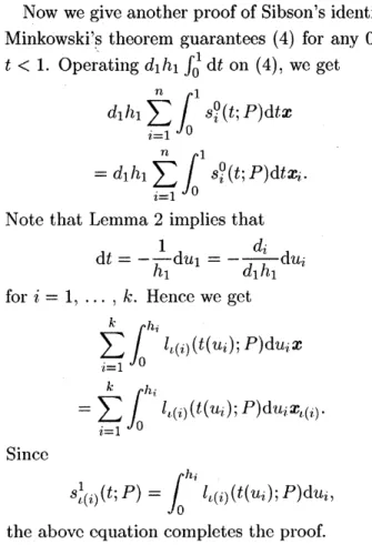
$P_{n}[3]$ ($cf$ Figure 3).

Figure4 shows

_an.example

of

a

surfaceobtained

from $\tilde{\varphi}^{0}$

.

Figure 3. Circles

on

which $\mathrm{C}^{2}$

-continuity of the

Sibson coordinates fails.

3

Another

_P.roof

of

Sibson’s

Identity

In this section,

we

give anotherproofofSibson’s

identity. Observing _{this proof closely leads to the}

this fact and Minkowski’s theorem, we get

Figure 4. An exampleofasurface obtained from

the Minkowski’s interpolant.

3.1

Proof

of the identity for the

Minkowski coordinates

At first, let us give a proof ofthe identity (2),

which comes from Hiyoshi-Sugihara [4]. For this

purpose, the following lcmma is used as a

funda-mental tool, which is known as Minkowski’s

the-orem:

Lemma 1 For any rcgion $V\subseteq \mathrm{R}^{d}$

.

the following

equation holds:

$\int_{Q\in\partial V}n\mathrm{d}S=0$, (3)

where $\partial V$ denotes the boundary

of

$V,$ $n$ denotes

the unit outer normal vector to $\partial V$ at $Q$, and$\mathrm{d}S$

denotes the

_{infinitesimal surface}

element at Q. $\square$

Let $P_{p(1)},$ $\ldots$ , $P_{\iota(k)}$ be the neighbors of the

tar-get point $P$

.

In general, the boundary of the

Voronoi region of some generator $Q$ is a

(possi-bly unbounded) polygon each edge of which is a

part of the perpendicular bisector of the line seg-ment $\overline{QQ’}$ with another generator $Q’$

.

Therefore,

the unit outer normal vector to the Voronoi edge

$E(P, P_{\iota}(i))$ is denoted by $(1/d_{L}))^{\frac{1}{PP_{\ell(i)}\prime}}(i$

.

$\mathrm{E}^{\backslash }\mathrm{o}\mathrm{m}$

$\sum_{i=1}^{k}\frac{l_{\iota(i)}}{d_{\iota(i\rangle}}=0\frac{1}{PP_{\iota(i)}\prime}$

.

Note that $l_{i}=0$ if $P_{i}$ is not a neighbor of $P$.

Hencewe get

$\sum_{i=1}^{n}\frac{l_{i}}{d_{i}}x=\sum_{i=1}^{n}\frac{l_{i}}{d_{i}}x_{?}.$

.

which proves (2).

3.2

Proof of Sibson’s

identity

Observing the proof we gave in Section 3.1

closely, we notice that the crucial fact is that for cach$P^{}\mathrm{s}$neighbor$P_{i}$, theVoronoiedge$E(P, P_{i})$ is

perpendicular to the vector $\frac{}{PF_{i}^{J}}$. Therefore, ifwe

find a polygoneach of whose edges is

perpendic-ular to the vector$\frac{}{PP_{i}}$ with someneighbor$P_{i}$, we

can obtain another coordinate $\mathrm{s}\mathrm{y}\mathrm{s}\mathrm{t}_{\mathrm{C}\mathrm{I}}\mathrm{n}$ from that

polygon.

At first, we describe a procedure for

construct-ing such polygons. Forthis purpose. the Voronoi

diagram $\mathcal{V}(P_{1}\ldots.’.P_{n}, P)$ is constructed. We

de-note$P\mathrm{s}$neighbors by

$P_{\iota(1)},$ _$\ldots,$ $P_{\iota(k)}$ inthe

coun-terclockwise order. Without loss of generality,

we assume that $P_{\iota(1)}$ is the nearest generator to

$P$ (choose arbitrary one if not unique).

Parti-tion $V(P)$ into the subregions $V(P.P_{\iota}(1\rangle)’\ldots$ , $V(P, P_{t(k)})$

.

Let $S_{i}\in\overline{V(P,P_{\iota})(i)}$bethe point

fur-thest from the line containing$E(P.P)\iota(i).\mathit{1}$ and let $t_{l_{i}}$ be the distance of $S_{i}$ from the line containing

$E(\dot{P}, P_{\iota(}i))$

.

Let

us

pay attention to $V(P, P_{t(1)})$

.

Since $P_{\iota(1)}$

is the nearest generator to $P,$ $\overline{V(P,P_{\iota(1\rangle})}$

con-tains the target point $P$. We start

construct-ing the polygon by strokconstruct-ing its first edge inside

$V(P, P_{\iota})(1)$. The following procedure outputs the

vertices ofa desired polygon.

1. Let $L_{1}$ be the line perpendicular to $\frac{\iota}{PP_{\iota(1)}\prime}$

suchthat $L_{1}\cap V(P, P_{\iota}(1))$ is not empty.

2. Let $\{Q_{1}, Q_{2}\}=\partial V(P, P_{\iota(1\rangle})\cap L_{1}$ sucll that

3. Set $\dot{i}\vdash 2$and_{$j\vdash 2$}

.

4. Let $L_{i}$ be the line that is perpendicular to

$\frac{\backslash }{PP_{L(i\rangle}\prime}$ and that contains

$Q_{i}$

.

5. If$L_{i}\cap V(P, P_{\iota(}i))$ is empty, go to

7.

6. Set$jarrow j+1$

.

Let $Q_{j}$ be the other endpoint

of the line segment $L_{i}\cap V(P, P_{t(i)})$

.

7. Set $\dot{i}\succ\dot{i}+1$

.

8. If$\dot{i}\leq k’$

.

go to 4. Otherwise output $Q_{1},$

$\ldots$ ,

$Q_{?}-1$ and terminate.

We denote the obtained polygon by $C(t)$, where

theparameteris determined in the following

man-ner. For$\dot{i}=1,$ $\ldots k_{t}\neq$

.

lct$u_{i}$denote the distance of

the line segments $V(P, P_{\iota})(i)\cap C(t)$, ifany. from

the Voronoi edge $E(P, P_{p(}i))$

.

Then, $t$ is set to

$(h_{1}-u_{1})/h_{1}$

.

It follows from the definition tllat

$0<t<1$

.

Note that $C(t)$ tends to the boundary

of $V(P)$ as $tarrow 1$

.

In fact, the abovc procedure

can be seenas the $\mathrm{i}\mathrm{n}\mathrm{c}\mathrm{l}\cdot \mathrm{C}m\mathrm{C}\mathrm{n}\mathrm{t}\mathrm{a}\mathrm{l}$algorithm for

con-structing Voronoi diagrams.

By setting $\partial V=C(i)$ in Lemma 1,

we

get the

following identity:

$\sum_{i=1}^{n}S_{i}(t;P0)x=\sum_{i=1}^{n}g_{i}(0P)t;xi_{J}$. (4)

where

$s_{i(;}^{0}tP)=l_{i}(t;P)/d_{i}(P)’$.

$l_{i}(t;P)=$ ($\mathrm{t}\mathrm{h}\mathrm{e}$length of

$C(t)\cap V(P_{i})$).

Wecall $s_{i}(0t;P)_{\mathrm{S}}$’ the weak Minkowski coordinates

with parameter $t$

.

Note that _{$s_{i}^{0}(t;P)arrow s_{i}^{0}(P)$} as

$tarrow 1$. Hence

we

define $s_{i}^{0}(1;P)=s_{i}^{0}(P)$ and

interpret $s_{i}^{0}(P)$ as the special _c\v{c}lse of the weak

Minkowski coordinates.

For the purpose of proving Sibson’s identity,we

require another fact. Let $e_{i}(t)$ denote the line

segment $V(P_{i})\cap C(t)$

.

Lemma 2 Two polygons $C(t)$ and $C(t+\mathrm{d}t)$

given,

assume

that the edges$e_{i}(t)_{!}$

.

$e_{i}(t+\mathrm{d}t),$ $ej(t)$,

and$e_{j}(t+\mathrm{d}t)$ exist. Let $\mathrm{d}u_{i}$ be the w\’idth between

Figure 5. Consecutive edges of $C(t)$ and $C(t+$

$\mathrm{d}t)$.

$e_{i}(t)$ and $c_{i}(t+\mathrm{d}t)$

.

and let $\mathrm{d}u$; be the width

be-tween $e_{j}(t)$ and $e_{j}(t+\mathrm{d}t)$

.

Then,

$d_{i}\mathrm{d}u_{i}=d_{j}\mathrm{d}u_{j}$

.

Proof. Let $b$ denote the perpendicular bisector

of the line scgment$\overline{P_{i}P_{j}}$

.

Then, theVoronoi edge

$E(P_{i}.P_{j})$ is a part of $b$

.

Let $\theta_{i}$ denote tlle angle

generatedbythe lines$b\mathrm{a}\mathrm{n}\mathrm{d}\overline{PP_{i}}$, and lct

$\theta_{j}$ denote

the angle generated by the lines$b$ and $\overline{PP_{j}}$

.

See

Figure 5.

It is clear that

$\frac{\mathrm{d}u_{i}}{\cos\theta_{i}}=\frac{\mathrm{d}u_{j}}{\cos\theta_{j}}$

.

Since$b\perp\overline{P_{i}P_{j}}$, the followingequations hold:

$\angle PP_{i}P_{j}=90^{0}-\theta_{i}$, $\angle PP_{j}P_{i}=90^{0}-\theta_{j}$

.

On the other hand, the sine theorem on the

tri-angle $PP_{i}P_{j}$ yields the equation $\frac{d_{j}}{\sin\angle PPiPj}=\frac{d_{i}}{\sin\angle PP_{j}P_{i}}$.

From the above equations,

we

get

$d_{i}\mathrm{d}u_{i}=d_{j}\mathrm{d}u_{j}$

.

Now wegive another proofof Sibson’s identity.

Minkowski’s theorem guarantees (4) for any $0<$

$t<1$

.

Operating $d_{1}h_{1} \int_{0}^{1}\mathrm{d}t$on (4), we get $d_{1}h_{1} \sum_{i=1}^{n}\int_{0}^{1}s_{i}^{0}(t;P)\mathrm{d}t_{X}$

$=d_{1}h_{1} \sum_{i=1}^{n}\int_{0}^{1}s_{i}^{0}(t;P)\mathrm{d}tx_{l}$.

Note that Lemma 2 implies that

$\mathrm{d}t=-\frac{1}{h_{1}}\mathrm{d}u_{1}=-\frac{d_{\mathrm{i}}}{d_{1}h_{1}}\mathrm{d}u_{i}$

for $\dot{i}=1,$ $\ldots$

,

$k$. Hence we get $\sum_{i=1}^{k^{\alpha}}\int_{0}h_{\dot{\tau}}l_{(i}(l)t(ui);P)\mathrm{d}u_{i}x$

$= \sum_{i=1}\int 0u_{i}khil_{p(i}()t();P)\mathrm{d}uiX(i)l$

.

Since

$s_{\iota(i)}^{1}(t;P \rangle=\int_{0}^{h_{i}}l_{\iota}(?.\rangle(t(u_{i});P)\mathrm{d}ui$,

the aboveeqllation completes tlle proof.

4

Generalization

of

Coordinate

Systems

Observing the proof given in Section 3.2

care-fully, we notice that Sibson’s coordinate system

is not the ollly one that we can obtain; other

co-ordinate systems can be obtained by modifying

the expression slightly. The followingare typical

lnodifications:

1. Any subinterval $(a, b)$ of$(0,1)$ is available as

the integration interval.

2. Furthermore,any interval $(a, b)$ with$0<a<$

$b$is available when we extend $C(t)$ naturally

for $t>1$

.

$C(t)$ with $t>1$ lies outside the

Voronoi regioll $V(P)$.

3. In the integration step, the weight function

$w(t)$ can be multiplied.

4. Multiple integration. We

can

construct other

coordinate systems by integrating previously

obtained coordinatesrepeatedly.

4.1

Standard

interpolants

Although a lot of coordinate systems

can

be

constructed by combining the above modifica-tions, we guess the following subclass of $s_{i}^{k}(P)$

is especially important. Each $k=0,1,$ $\ldots$

,

the

coordinate$s_{i}^{k}(P)$ is calculated in the following

re-cursion:

$s_{i}^{k}(P)=s_{i}^{k}(1;P)$

.

where

$s_{i}^{k}(t;P)=d_{1}h_{1} \int_{0}^{t}s_{i}h-1(s;P)\mathrm{d}S$ for $0<t<1$ .

We call $s_{i}^{k}(P)$ the order-k standard coordinates.

Minkowski’s coordinate system and$\mathrm{S}\mathrm{i}\mathrm{b}\mathrm{S}\mathrm{o}\mathrm{n}\mathrm{S}$

coor-dinate systemarethe$\mathrm{f}\mathrm{i}1^{\cdot}\mathrm{s}\mathrm{t}$twocoordinatesystems

in this subclass. The corresponding interpolant

$\tilde{\varphi}^{k}(P)=.\sum_{=?1}’ y_{i}s_{i}^{k}(P)l$ (5)

is called the order-k standard interpolant.

5

Computational

Experiment

In this section, we present some computational

results about the order-k standard interpolant.

Assume that the data$y_{j}=\delta_{ij}$ for sonle $\dot{i}=1$

.

.

. .

,

$n$ are given. Then we obtain the function

$\tilde{\varphi}^{k}(P)=\hat{s}_{i}^{k}(P)$ as the result. Therefore, we give

$\hat{s}_{i}^{k}$ the alias

‘

hat function”. The hat functionsare

important because the standard interpolant is a

linear combination of the hat functions.

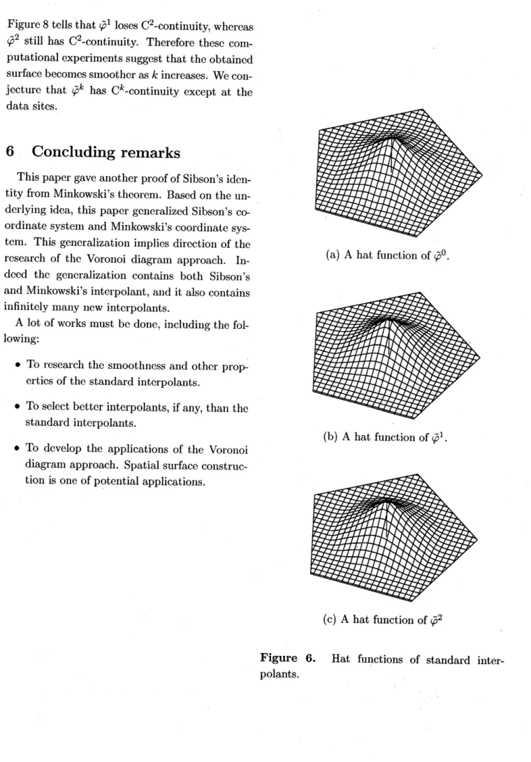
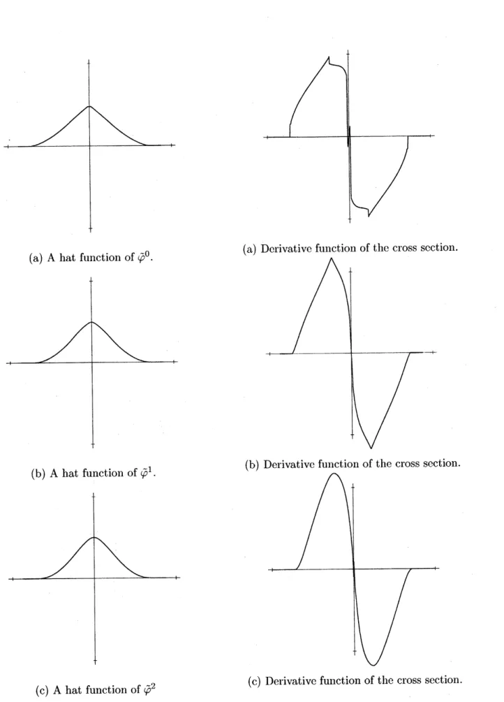
Figure6 describesexamplesof hat functions of

$\tilde{\varphi}^{0},\tilde{\varphi}^{1}$ and$\tilde{\varphi}^{2}$ for the datasites drawn in$\mathrm{F}\mathrm{i}\mathrm{g}\mathrm{U}1^{\backslash }\mathrm{e}3$

.

Although

our

eyes can hardly

see

the difference

among the figures. the following discussion clari-fies their difference.

Figure7describes thecrosssections of hat

func-tions cut by

a

vertical plane. Ifwe

see

the

cross

scction of $\tilde{\varphi}^{0}$, we notice that some non-smooth

points, as explained in Section 2. The slopcs of

these

cross

sections are drawn in Figure 8. The

Figure8 tellsthat$\tilde{\varphi}^{1}$ loses$\mathrm{C}^{2}$-continuity,

whereas

$\tilde{\varphi}^{2}$ still has $\mathrm{C}^{2}$

-continuity. Therefore these

com-putational experiments_{suggest that the obtained}

surfacebecomessmootheras $k$increases. We

con-jecture that $\tilde{\varphi}^{k}$ has $\mathrm{C}^{k}$

-continuity except at the

data sites.

6

Concluding

remarks

This

paper

gave anotherproofofSibson’s

iden-tity from Minkowski’s theorem. Based

on

the

un-derlyingidea, this paper generalized Sibson$\mathrm{s}$

co-ordinate system and Minkowski’scoordinate

sys-tem. This generalization implies direction of the

research of the Voronoi diagram approach.

In-deed the generalization contains both Sibson’s

and Minkowski’s interpolant, andit also contains

infinitely many new interpolants.

A lot of works must be done, including the

fol-lowing:

(a) A hat function of$\tilde{\varphi}^{0}$

.

$\bullet$ To research the smootllness

and other

prop-ertics of the standard interpolants.

$\bullet$ To select better interpolants, if

any,than the

standard interpolants.

$\bullet$ To develop the applications

of the Voronoi

diagram approach. _{Spatial surface}

construc-tionis one ofpotential applications.

(b) A hat function of$\tilde{\varphi}^{1}$

.

(c) A hat function of$\tilde{\varphi}^{2}$

Figure 6. Hat

functions

of standard

(a) A hat function of$\tilde{\varphi}^{0}$.

(b) A hat function of$\tilde{\varphi}^{1}$.

(c) A hat function of$\tilde{\varphi}^{2}$

(c) Derivative function of the

cross

section.

Figure 8. Derivative functions of the

cross

sec-Figure 7. Cross sections of hat functions.

References

[1] H. Edelsbrunner, Algorithms in

Combinato-rial Geometry, Springer-Verlag,Berlin, 1987.

[2] G. Farin, Surfaces

over

Dirichlet

tessella-tions, Computer Aided $Geometr\dot{i}c$ Design 7

(1990) 281-292.

[3] H. Hiyoshi and K. Sugihara, Another

inter-polant using Voronoi diagrams, IPSJ SIG

Notes 98-AL-62 (1998) 33-40, in Japanese.

[4] H. Hiyoshi and K. Sugihara, Two

generaliza-tions ofan intcrpolant basedon Voronoi

dia-grams, International Journal

_of

Shape

Mod-eling, to print.

[5] A. Okabe, B. Boots and K. Sugihara,

Spa-tial Tessellations: Concepts and Applications

of

Voronoi Diagrams, John Wiley

&Sons.

Chichester, 1992.

[6] F. P. PreparataandM. I. Shamos,

Computa-tional Geometry, Springer-Verlag,NewYork,

1985.

[7] B. Piper, Properties of local coordinates

based on Dirichlet tessellations, in G. Farin,

H. Hagen and H. Noltemeicr, eds.,

Geomet-ric Modelling, Springer-Verlag, Wien (1993) 227-239.

[8] R. Sibson, A _{vector identity for the}

Dirich-let tessellation, Mathematical Proceedings

_of

Cambridge Philosophical Society 87 (1980)

151-155.

[9] R. Sibson, A brief description of natural

neighbour interpolation, in V. Barnett, ed.,

.

Interpreting Multivariate Data, Johm Wiley

&Sons,

Chichester (1981) 21-36.

[10] K. Sugihara, Surface interpolation based on

new _{local coordinates, Computer-Aided}

De-sign 31 (1999) 51-58.

[11] A. H. Thiessen, Precipitation averages for

largc areas, Monthly Weather Report 39