Studies on Salinization of Groundwater (Part I) -Theoretical consideration on three-dimensional movement of salt water interface caused by the pumpage of confined groundwater in a fan-shaped alluvium-

奈良教育大学学術リポジトリNEAR

Studies on Salinization of Groundwater (Part I) ‑Theoretical consideration on

three‑dimensional movement of salt water interface caused by the pumpage of confined groundwater in a fan‑shaped alluvium‑

著者 FUKUO Yoshiaki, KISHI Yosuke, IKEDA Kazuhiro journal or

publication title

奈良教育大学紀要. 自然科学

volume 25

number 2

page range 13‑33

year 1976‑12‑25

URL http://hdl.handle.net/10105/2556

Studies on Salinization of Groundwater (Part I)

-Theoretical consideration on three-dimensional move- ment of salt water interface caused by the pumpage of corffined groundwater in a fan-shaped alluvium-

(With 8 Text-figures)

Yoshiaki FuKUof Yosuke Kishi** and Kazuhiro Ikeda***

(Received April 30, 1976)

Abstruct

Theoretical model is presented on the phenomena of sea water in- trusion into confined ground water, to make it clear the relationship between the pumping amount of fresh water and the corresponding spa- tial distribution of salt water in three-dimensional treatment. At first, the differential equations are derived in fresh and salinized regions, re- spectively, from the fundamental equation in confined water. The e- quation in salinized region, which is one of the quasi-linear differential equations, can be transformed to a linear one and then is continued to the equation in fresh region, resulting in the two-dimensional Poisson's equation which is been applicable to entire region. This equation in steady state is generally solved in integral form by using the method of Green's function and is simply expressed in the case of idealized field conditions analogous to a fan-shaped alluvium by the usual method of im- ages. Finally, some numerical examples are shown in the case of uni- form pumpage in a circular region.

1. Introduction

Recently it occurs often in our country that a large amount of ground water has carelessly consumed owing to the increasing demand for water due to the concentration of population and the progress of industrialization. Consumption of ground water has sometimes brought about the undesired phenomena such as the lowering of the water levels, the subsidence of ground surface and the intrusion of sea water into coastal aquifer. The phenomena of sea water intrusion into

Department of Geoscience, Nara University of Education.

Department of Applied Physics, Faculty of Engineering, Ehime University.

Science Laboratory, Suita High School, Osaka.

13

14 ^{Yoshiaki Fukuo, Yosuke Kishi} and Kazuhiro I keda

ground water is frequently seen in coastal regions, not only in large cities but also in small towns. In such regions, many wells near the coast are being aban- doned by the contamination of fresh water with salt water and it has resulted in trouble to the ground water utilization. In order to obtain a reasonable man- agement of its utilization, it is necessary with no doubt to make the quantitative estimation of suitable pumping amount of ground water. Analytical studies on the phenomena of sea water intrusion, taking the pumping amount of water into account, will certainly become helpful in establishing the available methods in the planning of ground water management.

In the aquifer near the coast, the intruding sea water may form a salt layer below the fresh warer because of its heavier density. Ghyben and Herzberg(1) were the first workers who studied on the interface between fresh and salt water. The variation of the interface in time was investigated by Bear and Dagan<2). Shamir and Dagan(3) studied on these phenomena in two-dimensional treatment, by solving numerically the differential equations of ground water move- ments. However in these studies, the relationship between the pumping amount of water and the corresponding distribution of salt layer thickness was not ade- quately taken into account. One of the authors'4'5' studied on these phenomena in two-dimensional treatment for both confined and unconfined ground water. In his papers, he adopted the approximation of hydrostatic pressure for ground water, movements and assumed the existence of sharp interface between fresh and salt water and, solving the equations in steady state, he obtained the relationship be- tween the pumping amount of water and the spatial distribution of salt water It is clear, however, that the two-dimensional treatment of ground water flow will give rise to some inconveniences and three-dimensional treatment is more de- sirable when applying his theory to practical problems with complicated field conditions.

In this paper, we shall attempt an extension of histheorysoas tobeapplicable to three-dimensional flow of ground water in confined aquifer and shall find out the method to obtain the steady state solutions of these phenomena under the complicated field conditions.

2. Derivation of Fundamental Equations

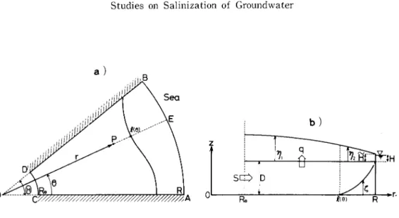
In order to investigate the phenomena of sea water intrusion into ground water, we adopt the theoretical model with idealized field conditions analogous to an alluvial fan as shown in Fig. 1,aand 1,b. Fig.1,a shows a plane view of field conditions. Confined ground water will flow in a fan-shaped area ABDC

with angle & and radius R. The positions in this area are denoted bycoordi-

Sea

ZV/////////////////////////////////////////^ ^£(ei

Fig. 1 a) A plane view of field conditions of our model.

b) A view of vertical cross section of our model.

nate (r, 6), the origin of which is on the top of the fan-shape. Ground water is supplied by uniform inflow through the arc CD at r = Ro and is dischargedinto

sea throughthearc AB at r-R. Bothsidewalls AC and BD ofthefan-

shaped area are regarded to be impervious boundaries, so the ground water will flow along them. If water is pumped from wells in this area, the pressure of ground water is lowered and sea water may seep through the arc AB along the lower surface of aquifer because of its heavier density. The seepage distances of salt water are designated by a curve r=£(9, t), depending on time t in general.

Fig. 1,b shows a view of vertical cross sectionofourmodel. Thez-axis is taken vertically upward as positive. We assume that the aquifer is homoge- neous and isotropic and has a constant thickness D everywhere, and postulate that the fresh water and salt water are immiscible and the two fluids are sepa- rated by a sharp interface z = £(r, 6, t) betweenthem. Attheboundary r=R where the aquifer is contact with the sea, the thickness of salt layer is chosen so as to coincide with that of aquifer D. As the radius 'r becomes smaller, the thickness of salt layer may decrease and tend to be zero at the distance r=£(6, t), the location of which will be called "the toe of interface between fresh and salt water". In the region Ro ^ r ^£{0,t), fresh water only exists and we shall call it "fresh region", while in the region £{d,t)^ r d,R, fresh water and salt water coexist and we shall call it "salinized region". The head of confined water is expressed as 7}i+D in fresh region and r)2+D in salinized region.

The fundamental equation of the ground water movements in confined aquifer

16 Yoshiaki Fukuo Yosuke Kishi and Kazuhiro Ikeda

is given by'^.(6)

dg> _ k(A

dt pigMA₉ ^(1),

where k is the hydraulic conductivity of aquifer, pi is the density of fresh water, A and fi are Lame's constants for the deformation of the aquifer and g is the gravitational acceleration, respectively. The <p is the piezometric head of ground warer which is defined by

Pig

(2),

where p is the pressure of ground water. If we express the Laplacian operator A in Eq. (1) by cylindrical coordinate, Eq. (1) is written as

32 ³ 2 32

I , 1 U i 1 f , C

Pig

>_k(A+2u)[d2 , 1 3 , 1

\ 3.,2 pis

)p (3).

3 fl 2 3~2

UU U <, I

Let us now consider the conditions at the boundaries of the confined aquifer.

The aquifer is generally bounded by upper surface z = %2(r,d,t) and lower one z = %i(r,d,t). The boundary condition at the upper surface is obtained by con- sidering a water balance in a small prismlike volume which is made at the upper surface z= f2 as is seen in Fig. 2. In this figure, thewater will flow intoor

q

T\ ^{å z=«2}

z=t

Fig. 2

Water balances in prismlike volumes made at the upper and lower surfaces.

out of this small volume through the sides and base of the prism. We assume that the ground water is sucked up through the upper surface of the aquifer by the amount q{r,d,t) per unit time per unit horizontal area. Conservation of water mass in this prism is given by the equation

<->ZT<i -U V*A

8r dd

where vr, ve and Vz are velocities of the ground water in the directions of r, 6 and z, respectively. Using the Darcy's law with respect to ground water flow

»= -&grad <p - (5),

we can write Eq.(4) as

__x_i£ a t z=%2 ^(6).

The boundary condition at the lower surface, which is treated as an impervious boundary, is obtained by similar way to the case of the condition at the upper surface. The result is

8 r dr r286 86 dz

d r dr r

1 d<p d£i d<p 2 36 99 ~8z

By integrating Eq. (3) with respect to z from

*t2 Zrr, ^('J_LO,,^r' /-?2f"/ 32

'"'I I II v

-II ll -

r Pig

d<p , _k(A+2u)

dt r ^dr1

to

+-T-r or at z=£1

f2 , it follows that

(7).

32

. 2 3d2 )<p \dz

r \j\j

(Pffll r 3fl, i

+^}^{dzlz=s2 -\^\^{{dz\z=tJ)z=UJ /a\}

Substituting the boundary conditions at the upper and lower surfaces Eqs.(6) and (7) into the above equation, we obtain

In the case where the slope of the aquifer is very gentle and ground water flows nearly horizontally, it may be reasonable to approximate the pressure of ground water p1 to be hydrostatic, that is,

pi =Pig{D+7)-z) (10).

Similarly the pressure of salt water p2 may be expressed as

p2 =P2g{D+H-z) (ll),

where p2 is the density of salt water and H is the height of sea level meas- ured from the upper surface of aquifer. Since the pressure-of fresh water must be equal to that of salt water at the interface z= %(r,d,t), we have

Pig(D+7j2-Z)=p2g(D+H-S) or

where

(D-S)=-y(jj2-H)

and Pi

Substituting Eq.(10) into (2), we obtain the piezometric head <p as for Ro^r^£(6,t), in freshregion

for £(6,t)^r ^R, in salinizedregion

<p-\

W+V2,

(12),

(13), (14),(15).

(16).

18 Yoshiaki Fukuo, Yosuke Kishi and Kazuhiro Ikeda

It is worthwhile to mention that we can obtain a simple expression in which the piezometric head <p becomes independent of coordinate z, owing to the approxi- mation of hydrostatic pressure of ground water. Furthermore, in our theoretical model shown in Fig. 1,aand 1,b, the upper and lower surfaces are put to be identical with those of the aquifer in fresh region, whereas the lower surface is chosen to be the interface between fresh and salt water in salinized region, that

?I= £2=D in both regions ^(17).

IS,

[.0 in fresh region I £ in salinized region

Substituting Eqs.(16) and (17) into (9), we thus obtain the fundamental equa- tions in unsteady state which describe the phenomena of sea water intrusion into coufined aquifer :

.dyi _ k(A+2/i)(d2

dt ^pig Xdr

i _i_A. J?yi

2 "T

dr

dt pig Idr{

+r2dd2 kD)

in fresh region (18),

-r>|p-}+-(0-?)#-_{b drJ r dr}

_L

dd

//.

W3rJ k)

in salinized region ^(19).

3. Continuation of Equations in Salinized and Fresh Regions

Eqs.(18) and (19) are time-dependent equations, the solutions of which may describe the variations of these phenomena in time but, in general, it may be dif- ficult to obtain such solutions. So, we will attempt to solve these problems in future and now restrict our argument in this paper to the steady state of these phenomena.

In steady state, we have the fundamental equations :

D dill. ₊

x^{r dvi.}_dr ^{+ 1} de2)^dyi\_. in fresh region ^(20),

a fK ^IH ^{j" Md-Z) df)2d r + ± _8_dd (D-OH }=}

in salinized region (21).

Boundary conditions in our model are expressed in terms of iji, r)2 and £ as follows ;

1) Ground water is supplied by the uniform inflow with the flowrate 5 through the arc CD :

dr kDRo 0 ^{at r=R0 (22),} 2) At r=R, the thickness of salt layer is equal to that of aquifer D :

£=D at r=R

or from Eq.(13)

7)2=H at r=R (23),

3) Ground water flows along the side Walls AC and BD of fan-shape :

3m-Mi.=o_{dd dd u at 6=0 and 6=6} ⁽²⁴⁾

4) At the toe of interface between fresh and salt water, 771 and 172 must be joined smoothly :

_ drjj__ dr[2_ drji _ drji

Vi~V2> dr~dr' dd~dd at r=£(6) ⁽²⁵⁾

Eq.(21) in salinized region, which is one of the quasilinear differential equa- tions, is transformed to a linear one in the following way.

Using Eq.(13),

-r\d22.=±(r,. - ff\d52_ =XjL (Xri.'- ff

W-SY^=^V2-H}_{dr y dr} y dr V2V2~H7i2)-lV[2 y i (26)>

and

(D- '

dd- dfi JV2-HY

dd\2 r

Eq. (21) becomes, therefore, a linear differential equation ( ^{d2 1 a . 1} da\[l(j2iiiH\2)=l

\3r2+rdr r2dd2){2\ 7D)J yr kD2

(27).

(28).

In fresh region, Eq.(20) is also rewritten as

/d2 1 3 1 3M/;

\dr2+rdr r2862)\

or

(_{3 .1-2} ^{i d l}_, ^{d2\(m-H 1}

Z 3/32I\ ^,n ^{~o~) tn^}

u/ r ui ' uu / \ /js a / / kls

(29).

It will be seen later why to subtract the constant one-half from the dependent variable. By introducing non-dimensional quantities 91*, V2* and q*, Eqs.(29) and (28) are expressed as

32 32

U i -L V

J r^{2 ' *å}

/ 32 1 d

\dr2

]

8 r ⁸⁸²

+ ^{i d2}

]Vl~D2

dd !^{) V2*=}

72"3fl2~/ '/2 D2r>2

u r r uu f js

respectively, where j?i*, rj2* and q* are defined by

(30),

(31),

20 Yoshiaki Fukuo, Yosuke Kishi and Kazuhiro Ikeda

m *= 1_TJr-H

2 yD

*-1.2-1(V2~H\2 Q ==J_JL

r k

(32), (33), (34).

We have thus obtained a formally identical linear differential equation both in sa- linized and fresh regions. In order to find out solution in both regions, it will be necessary to know how the solutions in one region is continued to that in an- other region at the boundary between them.

At theboundary r=£{6), %=0 and 71=92, so that the relation in Eq

(13) becomes

7?1 = r/2 =H+yD (35),

and then, the values of 771* and 7j2* are

that is

Vi =

T)i*- 7)2*-

.= l(T)2-_H\*==-H- 1 1

1/2 ⁰ \ å n I

iis f u

at r=£{0) ^(36).

Moreover, the first order derivatives of 771* and 772* with respect to r are

dr yD dr

and

dy2*_

d r ^h W\{7]2~H)^} -W^ _{at r=£(d)}

4) (Eq.(25))

at r=£(6) ^(37).

{rDY[ ^{\ '/2} dr) yD

and if follows that from the boundary condition 4) (Eq.(25) )

dr dr

Similarly,

^=-^ at r=4(8) (38).

Eqs.(36), (37) and (38) mean that rji* and rj2* are joined smoothly and that the value of rj* is always equal to 1/2 at the boundary of two regions,

r=£{6). We can, therefore, replace Eqs.(30) and (31) by a single equation which is common in both regions

"•Eå (&+*&+*&)'•E<'. «=*V1

with the boundary conditions 1'), 2') and 3') reexpressed in terms of v*

_1 S

1') 2') 3')

drf_ __

8r

?*=0

dd u

Ro&'

o* -- J-1

r kD2 ^{at r=R0 (40),(41),}

at r=R (42),

at 0=0 and 0=0 (43).

These boundary conditions are schematically shown in Fig. 3. The positions of

-

Afi } \dr~&8

J.--'- iW...J

Ro å =o

Fig. 3

Boundary conditions of v*(r, 8).

the toe of interface between fresh and salt water, r - £{6), are skillfully deter- mined by the equation :

V*{£(-8),8}= y (44).

and this is the reason why the constant one-half is subtracted from the depend- ent variable in fresh region.

4. Solutions of Laplace Equation by the Method of Green's Function In this section, we shall discuss the method to obtain the solutions of Eq.

(39) in the previous section which is the two-dimensional Laplace equation with sources q*(r, 6)1D2. The solution of Eq. (39) may be obtained in a integral form by the method of Green's function.

As is well known, the Green's function G(P,Q) is defined as one of the solutions of two-dimensional Laplace equation with a point source located at the position Q in the fan-shaped area :

APG{P, Q)=-d(P, Q) ^(45),

where P and Q represent the positions specified by the coordinates ( rP, dp) and (rQ, 8q), respectively, S(P, Q) is the two-dimensional delta function and dp is the Laplacian operator with respect to the position P. Then, the solution of Eq.(39) can be expressed as

V*{P) = -JL G{P' Q)<LW1doQ+7l0\P) _(46),

where the daQ is the surface element with respect to Q and the integration is carried out over the fan-shaped domain Do, and i)o*(P) is the solution in the absence of pumpage, i.e., a solution of a homogeneous Laplace equation

AP7]o*{P) =Q (47).

The function tj*(P) must satisfy the boundary conditions 1'), 2) and 3"

22 ^{Yoshiaki Fukuo, Yosuke Kishi and Kazuhiro Ikeda}

Then, it is natural that these conditions may be divided into two parts so that the one is satisfied by the function G(P, Q) and the other is satisfied by qo*(P) as is shown in the following :

1")

2")

3")

dn

s*

dG(P, Q),_n

dn "

Vo*(P)=Q G(P, Q)=0 dyo*(P) _n

--s~on"

dG(P, Q)

a t rP=Ra ^(48),

a t rP=R ^(49),

a t 6p=0 and 6P=Q ^(50),

where d/dn represents derivatives with respect to the point P in the directions normal to the boundaries.

It is worthwhile to mention that Eq.(46) holds even in more general case where the domain Do is bounded by an arbitrary closed curve. In that case, the boundary conditions are somewhat modified such a way that the derivatives d/dn appearing in Eqs.(48) and (50) are to be taken in the direction normal to the generalized boundaries. This fact allows us to extend our simple model rep- resented in Fig. 1, a ana 1,b to more generalized one which has a complicated plane-view as is the case with a real alluvial fan. Such an extension of our mod- el, which will be attempted in another occasion, may be useful when applying our model to practical problems.

In the simple case of fan-shaped area, the Green's function which satisfy conditions 1"), 2") and 3"), can be easily obtained by the usual method of images, as seen in Fig. 4. Starting from the source point Qi(r0, do) in the fan, we de- termine, at first, the position of its image point at Q2 with respect to the side OB of the fan. We further make, at theposition Q3, the imagepoint of Q2 with respect to the side OA' of the neighbouring fan OBA', and continue step by step to obtain finally the series of image points Qc(I=2, 3, •E•E•E,n) in a circle with the radius R. The number n must be an even integer in order to satisfy the condition that the image point of Qn with respect to the side OA should coin- cide with the source point Qi. This needs that theangle & of the fan is limited to

6>=^ (w=2,4,6, _(51).

We also obtain the series of inversion points Qi {l = 1, 2, 3, å •E•E,n) corresponding

to the points Qt(l=1, 2, 3, •Eå •E,n) with reference to the circle r =R, at the distance

r=L=- ^To

The above procedures are also shown in Fig. 4.

(52).

Fig. 4

Determination of image points and inversion points.

Now, we put positive unit discharges on each point Qi and negative unit discharges on Qi. The potential generated by a unit positive discharge at the position Q, which is one of the solutions of Eq. (45), is expressed at any point

P as

g (P, Q;a) &å «£å ^(53),

where ypq is the distance between the points P and Q, and a is an arbitrary constant. The Green's function G(P, Q), which satisfies boundary conditions

1"), 2"), and 3"), can be obtained by superposing the potentials of the forms of

Eq.(53) in which aconstant a ischosen tobe R and L for Qi and Qi,

respectively ,that is ,

G(P, Q)=]kg(P, Qi; R)-]tg(P, Q'f, L)

1 " J?2 1 n T2 1 " Iv2y'2\

where ri is the distance between P and Qi(n= r0) and r[ is the distance between P and Qi. Using the second cosine rule

rt2= r2+n2-2rorcos(d-dl)

24 Yoshia.ki Fukuo, Yosuke Kishi and Kazuhiro Ikeda

rt'2 = r2+L2-2Lrcos(d-di)

,R4 2R2r

=r -TTT2-_{r0 r0} cos(0-0t), wehave

C(P O)- X v1np.p?2+r°V/fl2-2rorcos(ff-&)l , ,

GiP, Q)-^21og| ro2+r2-2rorcoS(#-&) } (55)>

where r and 8 are thecoordinates ofthepoint P, 6\ and 6i{l=2, 3, •E•E•E,w) are angles of source point {di = do) and l-th image points, respectively which are given by

Ido ^{(/: odd)}

Ti-V<-i;c-r-j |6>-0o (I:even) v«-i,v" <s, o, å ", n> r^i

The function rjo*(P) is given by the potential generated by the positive dis- charge of magnitude S on the top of the fan i. e., origin of coordinate. From the boundary conditions 1"), 2") and 3"), we obtain

Vo\P) = Vo*(r) =f^\og^r _(57).

Substituting G(P, Q) and i?0*(P) thusdetermined into Eq. (46), weobtain the solution of Eq. (39), in the case of idealized field condition, as

L £ ff ^{Q*{n,,D2 do) log} R2+n2r2/R2-2nrcos (fl-flt)l

r o2+r2-2rorcos(0-0«) Jndnddo Introducing non-dimensional quantities

' -'i ^{r°~R' Q~D2q}

(58).

(59),

we can rewrite Eq.(58) as

7J*(r*, #) = 7T7a l0g"TT2

O* 1

26logV*

1 A ff n*(r. nUa,tt+ro*2r*2-2n*r*cos(d-di)) .,.,_,.

(60).

This is the solution of Eq.(39) which we want to obtain.

Once the solution has been obtained, the toe of interface between fresh and salt water is determined by the condition :

r)*{r*= l*(8), 6}=f (i*(e)= i(e)/R) ^(61).

Piezometric heads j?i and rj2 or <f>i and 4>i are obtained by the definitions (32) and (33):

* =*?#='•Eå for r* <L l*(6)

and

«52=^^=(2?*)^ for ne)±r*±\

The thickness of salt layer f is determined from Eq. (13) :

(62),

(63).

(64).

5. Numerical Examples

In this section, we shall give a numerical example in the simple case of uni- form pumpage in a circular region in the fan-shaped area. Let us now express Eq.(60) in the form :

? *(r\ fl)=g-log r^{1 1 n 1 "}

4 ff/=l 4ff/=l ^(65),

where

and

,/,= ff Q*(n*, 6o)\og{ro*2+r*2-2r0*r*cos(d-di)}r0*dro*ddo (66),

Ii = ff Q'iri, do)\og{l+ro*r*-2ro*r*cos(8-di)}n*dro*ddo (67).

JJDo

For the calculation of h, it is convenient that the integral variables (n*, do) in Eq.(66) are converted to new variables (b, 6') which have the origin at the center of the pumpage circle C, as shown in Fig. 5. 7i is then calculated as

Fig. 5

Transformation of integral variables

(r0*, do) tonew variables (b, 6') in

the calculation of

Ii.

J Jb. Q*(b, &') log( rP2+ b2-2brPcos 6')bdbdd'

6SC

X^cbdb - ^{fin,dd log(} rP2+bz-2brPcos 6')

'0

(68),

_Qo*

itc*

26 Yoshiaki Fukuo, Yosuke Kishi and Kazuhiro Ikeda

where Qo* is the total amount of pumpage in the circle which has the radius c, and rp is the distance between the position P(r*, d) and the center of the circle C. Now we have the integral formula (its derivation will be given in

Appendix )

0, if r^l

Anlogr, if r>1

Therefore, Eq.(68) should be calculated separately according to the case where the position P(r*, 6) is either outside the circle rp ^ c or inside the circle

rp<c.

a ) Inthecaseof rp^c;

r 2n fO if /-zi

/ Iog(l-2rcos#+r2)^= ' " \ (69).

Jo ^Axlos:r. if r>1

'' =$rw*r^10* -2+io^i+(^)2-fc°s ^"

r ^b_db ^{Cdd' he rp2}

n c'Jo Jo

=Qo*log rF2= Q0* \og{r*2+d2-2dr*cos (6-co)} (70),

where d and a> are the coordinates of the center of the circle C.

b) Inthecaseof rp<c;

n.* rrP r^n . . . .

h=^2 _JOI bdb _•E'OI dd'log(rP2+b2-2brPcos9)

_Qo*

,2

KC

+-^4 fCbdb f2"dd'log(rP2+b2-2brPcos 8')

7TC Jrp Jo

=Qo*^r\og rP2

+^4 fCbdb fVflog rP2+ log{l+W2-^cos 0D

KC JrP Jo \TPI Tp

=it^iá"2 l0g rp2+ frP bdMK hgJr]

= Q«^'I log c2-

1+ r*2+ d2-2dr*cos (6- co) _(71).

In the calculation of integrals M/^2) and 7/(/ ^l), the position P(r*, 6) is always outside the image circles, so results are similar to that of 7i where

rPhc:

L = Qo*\og{r*2+d2-2dr*cos{6-an)} (/^2)

(72),

Ii'= Qo* log{l+d2r*2-2dr*cos{6-coi)} (1^1) where coi is the angle of the center of the l-th image circle.

Summarizing these results, we obtain rj* in the case of uniform pumpage in a circle :

a) If the coordinate (r*, 6) is outside the circle, ri*(r*, 0)=glog^

-^iHog{l+d2r*2-2dr* cos (d-Wi)}

4K 1=1

+^jl \og{r*2+d2-2dr* cos {d-coi)}

b) If the coordinate (r*, 6) is inside the circle, V*{r*, 0)= g-log^

-^2 1og{l+</V2-2</r* cos (0-<y<)}

\K 1=1

(73),

+^{logc--l+^2+^-2^cos(g-^)}

+¥?-2 log[r*2+d2-2dr*cos (0-a;;)}

where

(Oi ==(1-1)0+ {^{(o (I : odd)}

(74),

(75).

(1=1 9 3 •E•E•E *,)

/ / . \

<vy-a> \i : even;

In Figs. 6,a - 6,j , we give some results of calculation of equi-potential lines of piezometric heads 4>\ and 4>z in the case where the angle 6 of fan is 60 degrees and the area of pumpage circle is 10 percent of total area of the fan (c=0.1291). The amount of inflow S* is fixed to 3.0 and the ratio of

a) b)

28 Yoshiaki Fukuo, Yosuke Kishi and Kazuhiro Ikeda

'Q2 ' 04 06 OS ' '1.P

Fig. 6 a)~h) ; Equi-potential lines of piezometric heads <l>\ and 4>z in the case of uniform pump-

age in acircle. The angle of fan 0=60 degree, radius of circle c=0.1291 andinflow-

rate S*=3.0.