NONUNIFORM WALL ZETA-POTENTIAL MEASURED BY

(1)

MICROCHANNEL WITH

NONUNIFORM WALL ZETA-POTENTIAL MEASURED BY

FLUORESCENCE IMAGING TECHNIQUE

by

Yutaka Kazoe

School of Integrated Design Engineering Graduate School of Science and Technology

Keio University

September 2008

(2)

(3)

Abstract

Microscale liquid flows under electric field, i.e., electroosmotic flows, have been widely used in the microscale flow systems: capillary electrophoresis system, and microfluidic devices such as micro total analysis systems and lab-on-a-chip. Electroosmotic flows are easily controlled by switching the electric field through electrode arrays, and useful for the miniaturization of systems by recent microfabrication techniques. However, the absence of two-dimensional measurement techniques for key parameters of electroosmotic flow, i.e., the time dependent flow velocity and the wall zeta-potential, has prevented experimental approaches to the flow with nonuniform wall zeta-potential by the material heterogeneity in a channel and the ion and thermal transport with mixing and chemical reaction. The present study developed a velocity measurement technique and a nanoscale laser induced fluorescence imaging for the zeta-potential measurement, and investigated electroosmotic flow with nonuniform wall zeta- potential. The momentum transport in the flow field and the eﬀect of the ion motion on the zeta-potential distribution were evaluated.

A time-resolved velocity measurement technique for transient electroosmotic flow was developed using fluorescent submicron particles and a high speed CMOS camera. Particle tracking velocimetry with low particle number density was employed in the present technique.

The high spatial resolution was achieved by an iterative measurement method based on the reproducibility of low Reynolds number flows. The combined measurement of near-wall and bulk velocities were realized by a measurement system using the evanescent wave and the volume illumination.

A novel measurement technique for nonuniform wall zeta-potential, termed nanoscale laser induced fluorescence imaging, was developed using fluorescent dye and the evanescent wave generated near the wall about 100 nm. The fluorescent dye, which ionizes in the electrolyte solution, was selected for the measurements. Since the fluorescence ions are distributed de- pending on the wall zeta-potential, the fluorescent intensity excited by the evanescent wave is related to the wall zeta-potential. An evanescent wave illumination system using two prisms was developed to achieve the large area measurement with the low magnification. The evanescent wave is generated using the microchannel substrates and prisms as an optical waveguide.

Transient electroosmotic flows in microchannels with uniform zeta-potential and nonuni-

(4)

form zeta-potential by material heterogeneity and the surface modification on the channel wall were examined using the developed velocity measurement technique. Electroosmotic flows with the channel scale of 10⁻⁴ m reached to the steady state at the time about 10⁻³ s after the electric field was applied. Electroosmotic flows have diﬀerent velocity profiles by the pattern and magnitude of wall zeta-potential, but the volumetric flow rate and the averaged zeta-potential shows a proportional relationship.

Electroosmotic flow with mixing of two electrolyte solutions at diﬀerent ion concentrations was investigated. The zeta-potential at the microchannel wall was measured by the nanoscale laser induced fluorescence imaging. The flow velocity was obtained using the conventional measurement technique, micron-resolution particle image velocimetry. The ion concentration in the flow field was estimated by the numerical analysis using the experimentally obtained velocity information. The measured zeta-potential distribution at the wall shows a quantitative relationship with the local ion concentration governed by the convection and diﬀusion with the mixing. Electroosmotic flow in the mixing flow field was induced by the zeta-potential distribution at the wall dependent on the ion motion.

The developed measurement techniques and the knowledge obtained from this work will contribute to the optimal design of the devices, the precise flow control technique using electrokinetics, and the novel applications such as mixing and separation by regulating the electric field and the zeta-potential.

(5)

List of Tables

2.1 Properties of water at T = 298 K . . . 17 2.2 Properties of ion species at T =298 K . . . 20 2.3 List of physical constants . . . 21 2.4 Properties of filter blocks for blue and green excitaiton (Nikon Corp.) . . . . 45 2.5 Specifications of the objective lenses (Nikon Corp.) . . . 47 2.6 Setups of the digital imaging devices . . . 47 3.1 Signal to noise ratios of the volume illumination images . . . 59 3.2 Random errors of particle displacement obtained by the PTV measurements. . 68 3.3 The maximum spatial resolutions and the measurement errors of PIV and the

iterative measurement using PTV . . . 72 3.4 List of parameters, uncertainties in 95% confidence level and the spatial reso-

lutions in the combined measurement of bulk and near-wall velocities . . . . 72 4.1 Properties of electrolyte solution . . . 87 4.2 The particle electrophoretic mobility,µep(m²/V s), and the zeta-potential at the

silica glass wall, ζ(V), with the measurement uncertainty in 95% confidence level obtained from 6 measurements . . . 92 5.1 List of uncertainties in 95% confidence level in the measurement of electroos-

motic velocity . . . 102

(10)

(11)

List of Figures

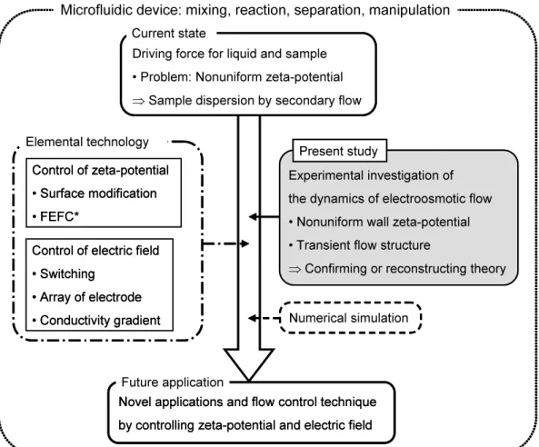
1.1 Schematic of electroosmotic flow induced by an external electric field. Parti- cles such as colloid and molecule is driven by electrophoresis. . . 2 1.2 Applications of electroosmotic flow to the microfluidic devices and contribu-

tion of the present study. . . 3 1.3 Objectives of the present study and outline of the dissertation. . . 10 1.4 Experimental approaches to electroosmotic flow in the present study. . . 11 1.5 Concept of the velocity measurement technique using tracer particles devel-

oped in the present study compared with the conventional techniques. . . 11 1.6 Concept of the zeta-potential measurement technique developed in the present

study compared with the conventional techniques. . . 12 2.1 (a) Schematic of the Couette flow between a fixed and a moving plate. (b)

Development of the Couette flow by the sudden acceleration of the plane to U₀(m/s) at t=0. . . 17 2.2 Geometry of a rectangular microchannel with the width of 2a (m), the depth

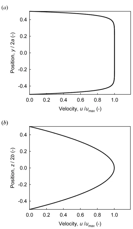
of 2b (m) and the length of l (m). . . . 18 2.3 Velocity profiles of pressure-driven flow in the rectangular microchannel with

k= 10 at (a) z/2b=0 and (b) y/2a= 0. . . 19 2.4 The diﬀusion coeﬃcient of the particle in the vicinity of the wall at T = 298

K (d_p = 500 nm, D= 9.79×10⁻¹³m²/s). . . 24 2.5 The theoretical model for the electric double layer, when the solid surface is

charged negatively. ψS (V) is the electrostatic potential at the solid surface. . 25 2.6 Velocity profile of electroosmotic flow at L/λD=100. . . 28 2.7 Schematic of particle electrophoresis with diﬀerent size compared to the De-

bye length. . . 28 2.8 Schematic of the polarized electric double layer around the particle on an ap-

plication of electric field. . . 30

(12)

2.9 Fabrication process of the microchannel by replica molding. (a) Master prepa- ration by photolithography. (b) Molding the microstructure to PDMS by replica molding. (c) Fabricating the microchannel used in the experiments. . . . 33 2.10 SEM images of PDMS microchannels fabricated by replica molding. . . 34 2.11 Schematic of SAM formed on the substrate. . . 36 2.12 Formation of SAMs by OTS on the glass surface through physisorption, hy-

drolysis in the adsorbed water layer, covalent binding to the glass surface and lateral polymerization with other OTSs. . . 37 2.13 Schematic outline of the process for microcontact printing of OTS to the glass

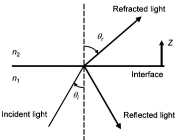
surface using a PDMS stamp. . . 38 2.14 Schematic of the energy-level diagram. . . 39 2.15 Schematic of refraction of light at an interface between two media of diﬀerent

refractive indices (n₁ >n₂). . . 41 2.16 Schematic of the evanescent wave generated by total internal reflection of light

at the interface. . . 41 2.17 The profiles of evanescent wave intensity at diﬀerent incident angles, when

the light ofλ=488 nm is totally reflected at an interface between borosilicate glass (n₁= 1.522) and water (n₂ =1.336). . . 42 2.18 Relationship between the incident angle and the penetration depth of the evanes-

cent wave, when the light of λ = 488 nm is totally reflected at an interface between borosilicate glass (n1 =1.522) and water (n2 = 1.336). . . 42 2.19 Schematic diagrams of (a) a fluorescence microscope and (b) an inverted flu-

orescence microscope. . . 44 2.20 Schematic of the recording optical system of the fluorescence microscope. . . 45 2.21 Schematics of (a) the objective lens-based TIRFM, and the prism-based TIRFMs,

in which (b) the prism is located in the opposite side toward the objective lens and (c) entry and exit prisms are located in the same side as the objective lens. 49 2.22 Schematics of (a) particle image velocimetry and (b) particle tracking ve-

locimetry. . . 51 3.1 Schematic diagram of the iteration measurement method using PTV. . . 56 3.2 Sample particle images with the volume illumination. The particle number

density is (a) 1.22×10¹⁰particles/ml and (b) 4.58×10¹⁰particles/ml. . . . . 58 3.3 Schematic of the near wall velocity measurement using the evanescent wave

illumination. . . 60 3.4 Sample images of fluorescent submicron particles with the evanescent wave

illumination. . . 60 3.5 Fluorescent particle illuminated by the evanescent wave. . . 61

(13)

3.6 Schematics of (a) the measurement system for investigations of transient elec- troosmotic flow, (b) the evanescent wave illumination and (c) the volume illu- mination in the microchannel. . . 63 3.7 Timing chart of the iterative measurement. . . 65 3.8 (a) Instantaneous vector map of the particle displacement during the time in-

terval of 400 µs obtained by PTV using the volume illuminaton images. (b) Instantaneous displacement vector map obtained after 6 iterative measurements. 66 3.9 Bias and random errors of PTV at the volume illumination evaluated using the

artificial images by the Monte Carlo simulation. . . 67 3.10 The time dependent particle displacements and the random errors obtained by

the PTV and the iterative measurement without the spatial averaging. The obtained displacements are at z = 26.4µm with the volume illumination and the number of iteration was 6. . . 69 3.11 The random errors of particle displacement by the spatial averaging at diﬀerent

vector numbers in the volume illumination (z = 26.4 µm) and the evanescent wave illumination. . . 70 3.12 The random errors by the spatial averaging at diﬀerent areas of the reference

region, when the number of iterative measurement was 6 and 12 in the volume and evanescent wave illuminations, respectively. . . 70 3.13 The random errors of PIV with the volume illumination and the evanescent

wave illumination at diﬀerent areas of the interrogation window. . . 71 3.14 (a) Side and (b) cross-sectional views of the glass microchannel. (c) Schematic

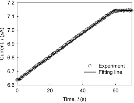
of the current monitoring setup. . . 73 3.15 The current profile with the time from the application of electric field, mea-

sured at the time resolution of 2 Hz. . . 74 4.1 (a) Schematic of the total internal reflection at the wall-liquid interface in the

microchannel. (b) Negative ion fluorescent dye and (c) positive ion fluores- cent dye in the vicinity of the wall surface with a negative zeta-potential is illuminated by the evanescent wave. . . 78 4.2 Structure of fluorescent dyes. (a) Alexa Fluor 546. (b) dichlorotris(1,10-

phenanthroline)ruthenium(II) hydrate. . . 81 4.3 (a) Schematic of the two-prism-based optical system for the evanescent wave

illumination in a microchannel. (b) Schematic of total internal reflections in- side the glass plate. . . 83 4.4 Schematic of (a) the experimental apparatus of the evanescent wave illumina-

tion system, (b) total internal reflection in the silica glass and (c) evanescent wave illumination in the microchannel. . . 85

(14)

4.5 Normalized intensity profile of the diﬀracted laser beam at the silica glass wall compared with the Gaussian intensity profile. The Gaussian intensity profile was calculated from the beam diameter of 0.65 mm estimated by the geometrical optics. . . 86 4.6 (a) Side and (b) cross-sectional views of the glass microchannel. (c) Schematic

of the closed cell. . . 88 4.7 Profile of particle velocity with standard deviation in the Z-direction in the

closed cell on an application of 10 V/cm. Dash line shows the fitting curve obtained by the least-squares method. Dash-dot-dot line shows the electrophoretic velocity calculated by equation (4.13). . . 90 4.8 (a) Side and (b) cross-sectional views of the silica glass channel. (c) Schematic

of the microchannel for the experiments. . . 90 4.9 Profile of electroosmotic velocity with standard deviation in the Z-direction in

the silica glass microchannel on an application of 20 V/cm. . . 91 4.10 Relationship between the bulk Na⁺concentration and the zeta-potential at the

silica glass wall. . . 91 4.11 Calibration curve between the corrected fluorescent intensity and the zeta-

potential. Error bars indicate the uncertainties of the zeta-potential as shown in table 4.2. . . 93 5.1 Two-dimensional channel with step change wall zeta-potential at y =0. . . . 97 5.2 Two-dimensional models for electroosmotic flow with nonuniform zeta-potential.

(a) Microchannel composed of walls with diﬀernent zeta-potential. (b) Mi- crochannel composed of walls with the zeta-potential distribution in the X- direction and uniform zeta-potential. . . 98 5.3 Schematics of microchannels (a) made of PDMS and (b) made of glass and

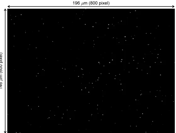
PDMS, and those with the OTS modification of the step pattern (c) perpendic- ular to the electric field and (d) parallel to the electric field. . . . 101 5.4 Evanescent wave illumination image of the surface modification pattern using

the Ru(Phen) solution. . . 103 5.5 Velocity vector maps at z = 39.6µm (a) in the center of the channel and (b)

near the side wall, when the microchannel was composed of PDMS walls. . . 105 5.6 Time-series electroosmotic velocity profiles in the Y-direction at z = 39.6µm

(a) in the center of the microchannel and (b) near the side wall, compared with the theoretical model. . . 106

(15)

5.7 (a) Depthwise velocity profiles of electroosmotic flow in the center of the channel, compared with the theoretical model. (b) Time-series measured and theoretical velocities at z = 39.6 µm, and errors of the measured velocities from the theoretical values and those by the approximation based on the central diﬀerence. . . 107 5.8 Near-wall velocity vector map at the glass wall, and velocity profile obtained

by averaging the velocities in the X-direction. . . . 109 5.9 Time dependent velocity profiles of electroosmotic flow in the depthwise di-

rection in the center of channel. . . 110 5.10 Spanwise velocity profiles of electroosmotic flow near the side wall at (a) z =

8.8µm, (b) z=39.6µm and (c) z=70.4µm. . . 111 5.11 Depthwise velocity profiles of electroosmotic flow at diﬀerent spanwise posi-

tions ((a) y=−342µm and (b) y=−250µm. . . 112 5.12 Near-wall velocity vector map with the step change zeta-potential perpendicu-

lar to the electric field, and velocity profile obtained by averaging the velocities in the X-direction. . . . 113 5.13 Streamwise velocity profiles in the YZ-plane at (a) t = 0.5 ms, (b) t = 1.3 ms

and (c) t= 7.7 ms. . . 115 5.14 Time-series velocity profiles of electroosmotic flow in the Y-direction at (a)

z=8.8µm, (b) z= 39.6µm and (c) z= 70.4µm. . . 116 5.15 Time-series electroosmotic velocity profiles in the Z-direction at (a) y = −75

µm (glass-PDMS), (b) y = −6.1 µm (glass-PDMS), (c) y = 8.6 µm (OTS- PDMS) and (d) y=77µm (OTS-PDMS). . . 117 5.16 Spanwise profiles of the shear stress on the fluid, τyx (Pa), at diﬀerent depth-

wise positions (t=7.7 ms), obtained from the velocity profiles. . . 118 5.17 Near-wall velocity vector map with the step change zeta-potential parallel to

the electric field, and velocity profile obtained by averaging the velocities in the Y-direction. Contours show the vector magnitudes. . . . 119 5.18 Velocity vector maps in the XZ-plane at (a) t= 0.5 ms, (b) t= 0.9 ms and (c)

t= 4.5 ms. Contours show the vector magnitudes. . . 121 5.19 Time-series depthwise velocity profiles in the X-direction at (a) z = 8.8µm,

(b) z =30.8µm and (c) z =52.8µm. . . 122 5.20 Time-series streamwise velocity profiles in the X-direction at (a) z = 8.8µm,

(b) z =30.8µm and (c) z =52.8µm. . . 123 5.21 Time-series electroosmotic velocity profiles in the Z-direction at (a) x=11µm

(glass-PDMS), (b) x= 84.3µm (glass-PDMS), (c) x=94.1µm (OTS-PDMS) and (d) y= 167µm (OTS-PDMS). . . 125

(16)

5.22 Streamwise profile of the pressure gradient at t =4.5 ms obtained by averaging over the depthwise direction,−d p/dx (Pa/m). . . 126 5.23 Streamwise profiles of the shear stress on the fluid,τxx(Pa), at diﬀerent depth-

wise positions (t= 4.5 ms), obtained from the velocity profiles. . . 127 5.24 (a) Volumetric flow rate normalized by that at the steady state with the normal-

ized time, t^∗ = t/τeo f (-). (b) Relationships between the averaged electroos- motic velocity and the average zeta-potential at diﬀerent times, t^∗(-). . . 129 6.1 (a) Top and (b) cross-sectional views of T-shaped microchannel. The thickness

of the silica glass was 1 mm for the nano-LIF imaging and 0.18 mm for the micro-PIV measurements. (c) Experimental setup for T-shaped microchannel. 132 6.2 Bulk concentration profile of Alexa Fluor 546 in the spanwise direction (Y-

direction) at x =200µm when U_ave =174µm/s. . . 134 6.3 Two-dimensional distributions of zeta-potential at the silica glass wall in the

junction area in (a) U_ave = 174µm/s and (b) U_ave = 420µm/s, respectively.

The DC voltage of 150 V was applied at t= 0. . . 135 6.4 (a) Velocity vector map at z = 26.4 µm obtained by micro-PIV. (b) Two-

dimensional distribution of Na⁺ concentration at z = 26.4 µm obtained by the numerical analysis using the micro-PIV results. The averaged velocity, U_ave, was 174µm/s. . . 137 6.5 Comparison of (a) zeta-potential profiles at the wall obtained by nano-LIF to

(b) Na⁺concentration profiles at z = 4.4µm and z = 26.4µm obtained by the numerical analysis in the Y-direction (x=150µm). . . 138 6.6 Relationship between the zeta-potential and Na⁺ concentration in U_ave = 174

µm/s and U_ave= 420µm/s. . . 139 6.7 (a) Velocity vector map in electrokinetic flow at z= 8.8µm induced by the DC

voltage of 150 V obtained by micro-PIV. (b) Profile of streamwise electroos- motic velocity at z = 8.8µm in the Y-direction (x = 400µm). The averaged velocity, U_ave, was 174µm/s. . . 141 6.8 Profiles of the electroosmotic mobility at the silica glass wall (z = 0), z = 8.8

µm, z = 26.4 µm and z = 44 µm (near the PDMS wall) in the Y-direction (x = 400 µm). The averaged velocity, U_ave, was (a) 174 µm/s and (b) 420 µm/s, respectively. . . 142

(17)

Nomenclature

Roman Symbols

a (m) half of channel width

A (m²) area

A_cross (m²) area of cross-section

A_total (m²) total area of wall in microchannel

b (m) half of channel depth

c (mol/m³) concentration c₀ (mol/m³) bulk concentration

c_f (mol/m³) fluorescence concentration

c_{f 0} (mol/m³) bulk concentration of fluorescent dye

C_D (-) drag coeﬃcient

d_e (m) eﬀective particle diameter captured on digital imaging device

d_p (m) diameter of particle

d_s (m) diameter of the diffraction-limited point spread function D (m²/s) diffusion coefficient

D_h (m) hydraulic diameter

Du (-) Dukhin number

D (m²/s) diﬀusion coeﬃcient tensor

e (m) smallest distance resolved by imaging device (pixel size) E_x (V/m) electric field in the X-direction

E_y (V/m) electric field in the Y-direction E_z (V/m) electric field in the Z-direction

E (V/m) electric field

f_E (N/m³) electric body force per unit volume f_obj (m) focal length of objective lens F (C/mol) Faraday’s constant

F (N) external force

(18)

FD (N) viscous drag force g (m/s²) gravitational acceleration

h (m) distance between the wall and the nearest edge of the particle

H_c (m) channel height

i (A/m²) current density

I₀ (W/m³) evanescent wave intentisy at interface I_e (W/m³) excitation light intensity

I_eva (W/m³) evanescent wave intensity I_f (W/m³) fluorescent intensity

j (mol/m²s) molar flux

k (-) aspect ratio of channel

k_b (J/K) Boltzmann constant

K (-) collection eﬃciency

Kn (-) Knudsen number

L (m) characteristic length

L_c (m) channel length

L_e (m) entrance length

m (kg) mass

L_s (m) length of sampling volume

M (-) total magnification of microscope

n (-) refractive index

n₁ (-) refractive index of first medium n₂ (-) refractive index of second medium

n_g (-) refractive index of glass

n_m (-) refractive index of immersing medium between objective lens and cover glass

n_s (-) refractive index of solution

N (-) number of particle velocities

NA (-) numerical aperture of objective lens

p (Pa) pressure

Pe (-) Peclet number

q (C) particle charge

q_E (C/m²) charge per unit area Q_2D (m²/s) two-dimensional flow rate Q_3D (m³/s) volumetric flow rate

r (-) correlation coeﬃcient

r_p (m) particle radius

(19)

R (J/mol K) gas constant

Roﬀ (m) oﬀ-center location of laser beam in the optical pathway of microscope

Re (-) Reynolds number

Re_p (-) particle Reynolds number

Sr (-) Strouhal number

t (s) time

t_c (s) time required for buﬀer exchange

t_g (m) thickness of glass plate

T (K) temperature

u (m/s) velocity in the X-direction u_cell (m/s) particle velocity in closed cell u_p (m/s) particle velocity

u (m/s) Velocity

U (m/s) characteristic velocity U₀ (m/s) initial velocity

U_ave (m/s) average velocity

v (m/s) velocity in the Y-direction w (m/s) velocity in the Z-direction

W_c (m) channel width

x (m) Cartesian coordinate in the streamwise direction

x (m) Spatial coordinate vector

y (m) Cartesian coordinate in the spanwise direction z (m) Cartesian coordinate in the depthwise direction

zv (-) ion valence

zvf (-) ion valence of fluorescent dye

z_p (m) penetration depth of the evanescent wave

Greek Symbols

α (°) half-angle of the maximum collection cone of light β (°) angle from the central axis of partice

χ (-) collection eﬃciency of the imaging device

δ (m) small distance

δp (m) penetration distance of diﬀusion

δz (m) depth of field of microscopic optical system

δzeva (m) measurement depth in the near-wall velocity measurement

(20)

δzm (m) measurement depth in the velocity measurement using tracer particle

∆t (s) time interval

∆x (m) displacement during the time interval

(C/V m) permittivity

0 (C/V m) permittivity of vacuum

m measurement error

r (-) relative permittivity

φ (-) quantum yield

γ (m²/mol) molar absorption coeﬃcient

η (m) position coordinate in particle

ϕ (°) inclination angle of laser beam

λ (m) wavelength

λD (m) Debye length

λl (m) length of the order of molecular diameter

λk (-) correction factor for the diffusion coefficient parallel to the λ_⊥ (-) wallcorrection factor for the diffusion coefficient perpendicular

to the wall

Λ (S m²/mol) molar conductivity

µ (Pa s) viscosity

µeo f (m²/V s) electroosmotic mobility µep (m²/V s) electrophoretic mobility ν (m²/s) kinematic viscosity

θ (°) angle

θc (°) critical angle

θi (°) incident angle

θp (°) incident angle at the prism-oil interface

θr (°) refractive angle

ρ (kg/m³) fluid density

ρE (C/m³) electric charge density ρp (kg/m³) particle density

σ (S/m) electrical conductivity

σs (S) surface conductivity

τ (s) charasteristic time

τ (Pa) shear stress

τc (s) convective time scale

τdl (s) charasteristic time for double-layer polarization

(21)

τeo f (s) charasteristic time for electroosmotic flow τep (s) charasteristic time for hydrodynamic relaxation

τp (s) particle relaxation time

τv (s) viscous time scale

υ (mol s/kg) mobility

ψ (V) electrostatic potential

ψS (V) electrostatic potential at solid surface

ζ (V) zeta-potential

Subscripts

ave average value

eva excited by the evanescent wave

eo f electroosmotic flow

ep electrophoresis

i ith

max maximum value

p particle

pre pressure-driven flow

re f reference

vol excited by the volume illumination

k parallel to the wall

⊥ perpendicular to the wall

+ positive ion

− negative ion

Superscripts

∗ dimensionless variable

Mathematical

h i time average value

(22)

(23)

Chapter 1 Introduction and Objectives

1.1 Introduction

Microscale fluid flows are observed in blood capillaries and microorganisms (biological field), porous media like mineral substrates (geophysical field), and industrial applications: ink-jet nozzles, capillary electrophoresis (Li, 1992; Quigley & Dovichi, 2004; Ghosal, 2006), electrical chromatography (Heftmann, 1992), and microfluidic devices such as micro total analysis systems and lab-on-a-chip (Geschke et al., 2004; Vilkner et al., 2004; Stone et al., 2004;

Dittrich & Manz, 2006). They are generally laminar flows, and interfaces between fluids (solid-liquid, liquid-liquid, gas-liquid) are stably existing since the surface tension is domi- nant. Especially, microscale liquid flows under electric field, i.e., electroosmotic flows, have been used as driving forces of liquids and samples in the electrochemical and biochemical applications. Since electric circuits are easily miniaturized by recent micro fabrication techniques developed in micro electro mechanical systems (MEMS), electroosmotic flows are useful for the microscale flow systems alternative to microscale pressure-driven flows, which require mechanical pumps and valves preventing miniaturization, and larger pressure loss than the macroscale flow systems (Dutta et al., 2006).

Electroosmotic flows are generated by the electric body force exerted on the liquid, and typical flow velocities are up to 1 cm/s. Figure 1.1 illustrates the schematic diagram of electroosmotic flow. When the liquid is filled in the channel, surface of the channel wall is charged, and near-wall region is electrically polarized by attracted ions with opposite charge to the wall, i.e., the electric double layer with a thickness about 1 ∼ 10 nm (Probstein, 1994; Lyklema, 1995). Hence, the liquid is driven by the drag of ions in the electric double layer migrated under the electric field. The flow velocity is proportional to the magnitude of electric field due to the electric body force, and the flow direction is easily controlled by switching the electric field. The electric body force also depends on the magnitude of near-wall electric

(24)

Electrophoresis (colloid, molecule) Electroosmotic flow

1 ~ 10 nm Electrophoresis (colloid, molecule) Electroosmotic flow

1 ~ 10 nm

Figure 1.1. Schematic of electroosmotic flow induced by an external electric field. Particles such as colloid and molecule is driven by electrophoresis.

polarization, which is determined by the electric charge at the wall characterized by the zeta- potential (Hunter, 1981; Kirby & Hasselbrink, 2004a,b). In the channel with the scale of 10⁻⁴m (microchannel), the thickness of the electric double layer is generally negligible compared with the channel scale. Only the near-wall region (inside the electric double layer) is dominated by viscous and electrostatic forces, while the bulk region is dominated by vicous and inertial forces. Thus, electroosmotic flows in the bulk region are described using the slip boundary condition with a velocity at a plane separating near-wall and bulk regions. When the wall charge characterized by the zeta-potential is uniform, the slip velocity is given by the Helmholtz-Smoluchowski equation, u_{eo f} = −ζE/µwhere u_{eo f} (m/s) is the electroosmotic velocity, (C/V m) is the liquid permittivity, ζ(V) is the wall zeta-potential, E (V/cm) is the electric field magnitude and µ (Pa s) is the liquid viscosity. In addition, if all the channel walls have a same zeta-potential, electroosmotic flow in the bulk region has uniform velocity profile, i.e., the plug flow (Probstein, 1994). On the other hand, particles such as colloids and molecules suspended in the liquid have own charges and migrate under the electric field, i.e., electrophoresis (Probstein, 1994; Lyklema, 1995). The flows involving electroosmotic flow and electrophoresis are termed electrokinetic flows.

Figure 1.2 shows applications of electroosmotic flow to the microfluidic devices and contribution of the present study. Electroosmotic flows have been used in various applications of the microfluidic devices: capillary electrophoresis microchip (Harrison et al., 1992, 1993;

Jacobson et al., 1994; Chabinyc et al., 2001), cell sorting (Li & Harrison, 1997; Sun et al., 2007), cell lysis (Lee & Cho, 2007), micro-reactors (Fletcher et al., 2001; Nelstrop et al., 2001; Debusschere et al., 2003), pumping and flow switching (Seller et al., 1994; Wu et al., 2007), sample stacking (Osbourn et al., 2000; Jung et al., 2003), mixing (Oddy & Santiago, 2001; Lin et al., 2004; Leong et al., 2007) and separation (Devasenathipathy et al., 2003).

(25)

Microfluidic device: mixing, reaction, separation, manipulation

Control of zeta-potential

• Surface modification

• FEFC*

Driving force for liquid and sample

• Problem: Nonuniform zeta-potential

⇒

Sample dispersion by secondary flow

Control of electric field

• Switching

• Array of electrode

• Conductivity gradient

Experimental investigation of the dynamics of electroosmotic flow

• Nonuniform wall zeta-potential

• Transient flow structure

⇒

Confirming or reconstructing theory Present study

Elemental technology

Novel applications and flow control technique by controlling zeta-potential and electric field

*: field-effect flow control (FEFC)

Numerical simulation Current state

Future application

Microfluidic device: mixing, reaction, separation, manipulation

Control of zeta-potential

• Surface modification

• FEFC*

Driving force for liquid and sample

• Problem: Nonuniform zeta-potential

⇒

Sample dispersion by secondary flow

Control of electric field

• Switching

• Array of electrode

• Conductivity gradient

Experimental investigation of the dynamics of electroosmotic flow

• Nonuniform wall zeta-potential

• Transient flow structure

⇒

Confirming or reconstructing theory Present study

Elemental technology

Novel applications and flow control technique by controlling zeta-potential and electric field

*: field-effect flow control (FEFC)

Numerical simulation Current state

Future application

Figure 1.2. Applications of electroosmotic flow to the microfluidic devices and contribution of the present study.

(26)

Several applications using electrokinetics are achieved by temporally regulating the electric field. The flows with the plug profile eﬀectively transport the samples without the advective dispersion compared with pressure-driven flows with the parabolic profile. Furthermore, the separation of samples by their own charges is easily achieved due to electrophoresis in electrokinetic flows. However, there is a critical problem that the wall zeta-potential is often nonuniform in the devices with practical application. Generally, the zeta-potential strongly depends on the ion concentration, pH and temperature of the liquid and the material properties (Kirby & Hasselbrink, 2004a,b). Thus, the nonuniform zeta-potential occurs in microfludic devices by the ion transport with mixing (Shinohara et al., 2004, 2005) and chemical reaction (Baroud et al., 2003; Ichiyanagi et al., 2007), the thermal transport with mixing (Sato et al., 2003b) and the Joule heating (Erickson et al., 2003), heterogeneity of materials in the mi- crochannel, and the surface chemical modification to the wall avoiding sample adhesion and controlling wettability (Whitesides et al., 2001; Pallandre et al., 2006). This heterogeneous wall zeta-potential significantly aﬀects the flow profile and flow rate of electroosmotic flow, and unexpectedly changes the sample dispersion and quantity of products in the chemical reaction. In contrast, several works have made attempts to control the electroosmotic flow profile and the sample dispersion in the microchannel by controlling the local zeta-potential at the channel wall. A typical approach to control the wall zeta-potential is the surface modification by coating or patterning. Electroosmotic flows with opposite directions in the same channel or recirculating flow profiles have been generated by coating or patterning chemical materials on the channel wall to change the zeta-potential (Barker et al., 2000; Stroock et al., 2000;

Stroock & Whitesides, 2003). Another approach is using a technique for the dynamic control of wall zeta-potential, i.e., field-eﬀect flow control (FEFC) developed by Schasfoort et al.

(1999). FEFC modifies the wall zeta-potential using a transverse electric field applied through the insulating microchannel wall. The voltage applied from an electrode embedded inside the wall increases or decreases the zeta-potential without aﬀecting the axial electric field to gener- ate electroosmotic flow (Buch et al., 2001). Suppressing the sample dispersion in a U-shaped microchannel (Lee et al., 2004), flow switching (Sniadecki et al., 2004) and enhanced mixing (Wu & Liu, 2005) were achieved by spatial and temporal control of local electroosmotic flow using FEFC.

The dynamics of steady and transient electroosmotic flows at the nonuniform wall zeta- potential is fundamental for the development of microfluidic devices. Numerical simulation using the current theory has been conducted to understand the structure of electroosmotic flow with the nonuniform wall zeta-potential (Ajdari, 1995; Ren & Li, 2001; Erickson & Li, 2003;

Fu et al., 2003; Park et al., 2007). Since the approximation using the Helmholtz-Smoluchowski equation can not be applied when the wall zeta-potential is inhomogeneous, the mass transport of charged species in the electric double layer must be considered to obtain the near-wall flow

(27)

structure. However, it is diﬃcult to estimate the mass transport in the electric double layer of 1 ∼ 10 nm thickness due to the resolution of numerical simulation in the microchannel. In addition, there is a question on the continuum assumption of fluid flow in such a nanometer order scale. Thus, experimental approaches are strongly required to confirm or reconstruct the current theory, and to realize a novel application and a flow control technique by regulating the wall zeta-potential and the electric field in the microchannel.

The present study experimentally investigates electroosmotic flow with nonuniform wall zeta-potential. Key elements for the experimental approaches are (i) time-resolved velocity measurement of transient electroosmotic flow, (ii) near-wall velocity measurement and (iii) measurement of the spatial and temporal distribution of wall zeta-potential.

1.2 Literature Survey

This section examines previous work related to the present study focusing on measurement techniques for the electroosmotic velocity and the wall zeta-potential, and experimental investigations of electroosmotic flow with nonuniform zeta-potential.

1.2.1 Velocity Measurement of Electroosmotic Flow

A method for the velocity measurement of electroosmotic flow is the current monitoring tech- nique proposed by Huang et al. (1988). The electroosmotic velocity is obtained by measuring a time required for the current in the microchannel to be plateau with exchanging an electrolyte solution to another at a slightly different concentration, which is proportional to the electrical conductivity of solution. Spehar et al. (2003) measured the electroosmotic mobili- ties,µeo f =u_{eo f}/E (m²/V s), in the microchannels made of fused silica, poly(dimethylsiloxane) (PDMS), and PDMS and glass (heterogeneous material) at different pH and electrolyte con- centrations. Liu et al. (2000) conducted the measurements using the microchannels coated by polyelectrolyte multilayers and evaluated the electroosmotic mobilities at different pH. Since the obtained electroosmotic velocity or mobility is the averaged value along the microchannel, major application of this technique is evaluating the electrokinetic characteristic of the microchannel rather than investigating the electroosmotic flow structure.

Spatially-resolved velocity measurements using flow tracers such as dye and particles (Sin- ton, 2004) have been conducted to examine the electroosmotic flow field in the microchannel.

Minor et al. (1997) measured the velocity of silicon iodide particles in electrokinetic flow in a closed 2 mm diameter capillary using laser Doppler velocimetry (LDV), which is a conventional technique for macroscale flow. However, it is diﬃcult to achieve a micrometer order spatial resolution by LDV due to the size of probe volume. Tsuda et al. (1993) and Taylor

(28)

& Yeung (1993) performed the flow imaging using a fluorescent dye by monitoring the front of fluorescence-labeled solvent in the capillary. The interface between the labeled and non- labeled solutions was significantly blurred due to the diﬀusion of fluorescent molecules along the capillary, and thus this technique did not achieve the quantitative measurement of velocity profile. Taylor & Yeung (1993) also examined electrokinetic flow using fluorescent submicron particles and a CCD camera, and roughly estimated a velocity profile from captured particle streaks resulting from the motion of particles during a single exposure. However, the velocity of electroosmotic flow was not obtained because the motion of particles in electrokinetic flow is the superposition of electroosmotic and electrophoretic components.

Paul et al. (1998) developed a velocity measurement technique using a caged fluorescent dye, and performed the measurement in a fused-silica capillary. An ultraviolet laser pulse is irradiated to generate a fluorescence-tagging pattern into the flow by uncaging the fluorescent dye. The velocity profile is obtained from the transport and distortion of the uncaged region. The electroosmotic velocity is estimated by subtracting the electrophoretic velocity of dye from the observed velocity. Ross et al. (2001b) conducted the measurement using caged fluorescent dye in plastic microchannels. Sinton et al. (2002) measured the electroosmotic velocities in a capillary, which quantitatively agreed with the results obtained by the current monitoring. Sinton & Li (2003) investigated electroosmotic velocity profiles in microchannels of circular and rectangular shapes at diﬀerent channel scales. Mosier et al. (2002) developed a photobleached-fluorescence imaging technique for microchannel flow. The photobleached region of the fluorescent dye solution in the microchannel is traced to obtain the flow velocity.

These dye-based techniques, called molecular tagging velocimetry, is a strong method for the quantitative velocity measurement for electroosmotic flow. However, the measurement error is significantly increased in the flow with large velocity gradients due to the advective dispersion of dye caused by the shear rate. In addition, the depthwise resolution of the measurement is relatively low due to out-of-focus fluorescence.

Micron-resolution particle image velocimetry (micro-PIV) proposed by Santiago et al.

(1998) is a most broadly used technique for the spatially-resolved velocity measurement in the microchannel. Microscopic images of fluorescent particles suspended in the liquid are captured by a digital imaging device, and the flow velocity is obtained by tracing patterns of particles in interrogation regions. Kim et al. (2002) conducted the micro-PIV measurement in electrokinetic flow in a T-junction microchannel made of PDMS, and compared the velocity profiles with those obtained by the numerical simulation. Devasenathipathy & Santiago (2002) firstly measured the electroosmotic velocity using micro-PIV by subtracting the electrophoretic velocity of particles from the observed velocities. Measurements were performed using an acrylic cross-microchannel and a microchannel composed of PDMS and glass, and the electroosmotic mobilities at material surface were obtained. Ichiyanagi et al. (2005) measured

(29)

electroosmotic velocity in a microchannel composed of PDMS and glass, and investigated electroosmotic flow with exchange of a buﬀer solution to another at diﬀerent pH. Sasaki &

Sato (2006) evaluated the eﬀect of surface modification to the microchannel wall on electroosmotic flow. In standard micro-PIV, the instantaneous velocities are temporally averaged to eliminate an error due to the Brownian motion of tracer particles, thus the measurement object is limited to the steady flow. On the other hand, Yan et al. (2006) examined transient elec- troosmotic flow in a submillimeter channel made of glass by using time-resolved micro-PIV.

Although the measurement error due to the Brownian motion remained, the transient structure of electroosmotic flow with homogeneous zeta-potential was firstly obtained. They also examined transient electroosmotic flow in a closed channel (Yan et al., 2007).

In order to investigate the near-wall structure of electroosmotic flow, Sadr et al. (2004) and Sadr et al. (2006) measured the velocity of electroosmotic flow in the vicinity of glass wall in a microchannel by nano-particle image velocimetry (nano-PIV). Nano-PIV enables the near-wall velocity measurement by using the evanescent wave generated by the total internal reflection of laser beam at the wall-solution interface (Zettner & Yoda, 2003). The evanescent wave is a light decaying exponentially from the wall with the order of 100 nm, and illuminates the tracer particles only in the vicinity of the wall. The near-wall electroosmotic mobilities were obtained from the measurement results, but the spatial resolution and the measurement accuracy are lower than micro-PIV due to escape of tracer particles from very thin illumination area by the Brownian motion.

For a turbid media where the spatially-resolved velocity measurement techniques based on the fluorescence imaging can not be applied, Wang et al. (2004a,b) developed phase-resolved optical Doppler tomography and conducted velocity measurements of electroosmotic flow in a microchannel. The cross-sectional velocity profile was obtained by collecting the back- scattered light from tracer particles at diﬀerent depths through an objective lens.

1.2.2 Measurement of Wall Zeta-Potential

Measurement techniques for the zeta-potential at a solid-liquid interface has been mainly based on electrophoresis of particles suspended in the liquid in a closed cell (Probstein, 1994; Hunter, 1981; Minor et al., 1997; Mori & Okamoto, 1980). A method for the zeta-potential measure- ment using a sound wave induced by oscillating motion of particles due to electrophoresis in AC electric field was also proposed (Carasso et al., 1995; Walldal, 2001). Oddy & Santiago (2004) developed a measurement technique for electrophoretic and electroosmotic mobilities using the particle displacements in AC and DC electric field.

A conventional technique for measuring the wall zeta-potential is the streaming potential measurement (Oldham et al., 1963). Streaming potential is an electric potential related to the wall zeta-potential, induced by the motion of diﬀused ions in the electric double layer actuated

(30)

by a high pressure applied into a channel. van Wagenen et al. (1981) evaluated the wall zeta- potential of various polymer materials. Scales et al. (1992) investigated the zeta-potential at the silica glass wall at diﬀerent pH and electrolyte concentrations, and analyzed the results on the basis of a theoretical model of the electric double layer. In principle, the zeta-potential obtained by the steaming potential measurement is spatially averaged value in the channel.

Recent studies have measured the electroosmotic velocity or mobility, and estimated the wall zeta-potential using the Helmholtz-Smoluchowski equation, ζ = −(µ/E)u_{eo f} or ζ =

−(µ/)µeo f. Sinton et al. (2002) evaluated the wall zeta-potential in the capillary from the electroosmotic velocity measured by the technique using the caged fluorescent dye. However, since the caged fluorescent dye significantly adsorbs to polymer materials and aﬀects the wall zeta-potential, this technique is unsuitable for the zeta-potential measurement in polymer mi- crochannels (Ross & Locascio, 2003). Sze et al. (2003) measured the zeta-potential at glass and PDMS surfaces by the current monitoring technique. Because of the current monitoring technique to measure the average velocity of electroosmotic flow, the obtained zeta-potetnial is also the spatially averaged value in the microchannel. Ichiyanagi et al. (2005) and Sasaki

& Sato (2006) estimated the wall zeta-potential from the electroosmotic velocity measured by micro-PIV. Even in the microchannel composed of diﬀerent materials, the wall zeta-potential can be evaluated by measuring the electroosmotic velocity near the each wall. However, due to use of the Helmholtz-Smoluchowski equation, the measurement regions are restricted to areas where the zeta-potential is assumed to be uniform at the wall. On the other hand, Park & Lee (2007) proposed a method estimating an inhomogeneous wall zeta-potential from the measured electroosmotic velocities, by solving the inverse problem using the governing equations for electroosmotic flow. This method was examined by the simulated velocity measurements but has not been applied to the real experiments.

1.2.3 Experimental Investigation of Electroosmotic Flow with Nonuni- form Zeta-Potential

Herr et al. (2000) coupled two capillaries to generate an axial distribution of wall zeta-potential, and examined electroosmotic flow and the sample dispersion by the velocity measurement technique using the caged fluorescent dye. An internal pressure was generated by the axial variation of wall zeta-potential, and aﬀected the flow profile and the dye dispersion.

Barker et al. (2000) modified the channel wall by polyelectrolytes to induce the step change zeta-potential along a direction perpendicular to the electric field, and generated a flow in opposite directions in the same channel. The sample dispersion and the motion of particles were observed by the flow imaging using the caged fluorescent dye and the velocity measurement using the streaks of fluorescent particles, respectively.

(31)

Stroock et al. (2000) and Stroock & Whitesides (2003) conducted the velocity measure- ment using particle streaks to examine the flows with the step change zeta-potential perpendicular and parallel to the electric field. The step change zeta-potential perpendicular to the electric field generated the co-flows in opposite directions as same as Barker et al. (2000), and the step change zeta-potential varying parallel to the electric field generated a recirculating flow profile.

Krishnamoorthy et al. (2006) experimentally and numerically investigated the structure of electroosmotic flow with nonuniform wall zeta-potential patterned by surface oxidation procedures. The mass flow rate obtained by the current monitoring and the sample dispersion calculated by the numerical simulation were aﬀected by the magnitude of surface oxidation.

Horiuchi & Dutta (2006) conducted the micro-PIV measurement to investigate electroosmotic flow controlled by FEFC, and developed a flow control device using a T-junction microchannel.

1.3 Motivation and Objectives

The motivation of the present study is to experimentally investigate the dynamics of electroosmotic flow in a microchannel with nonuniform wall zeta-potential. The key parameters for the investigation are the wall zeta-potential, the near-wall velocity by the zeta-potential and the time dependent bulk flow velocity. In the current state, experimental studies are limited to steady electroosmotic flow with typical patterns of surface modification or FEFC, where the distribution of wall zeta-potential is easily predicted. A critical problem is the absence of measurement techniques for the quantitative evaluation of the key parameters. The absence of the measurement technique for inhomogeneous wall zeta-potential prevents the investigation of flows with mixing and chemical reaction, in which the wall zeta-potential will distribute by the ion and thermal transport in the flow field. Investigations of near-wall flow structure are indispensable to evaluate the eﬀect of nonuniform wall zeta-potential on the flow field through the electric body force. Examing the transient flow structure leads to understand the momentum transport to form the flow field.

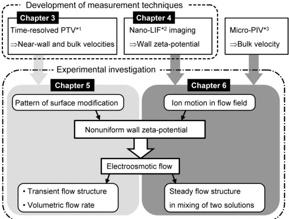
Figure 1.3 depicts the objectives of the present study and outline of the dissertation. The objective of the present study is to develop measurement techniques based on fluorescence imaging for the flow velocity and the wall zeta-potential. These techniques enable the time- resolved combined measurement of near-wall and bulk flow velocities, and the two-dimensional measurement of wall zeta-potential. Another objective is to investigate electroosmotic microchannel flow with nonuniform wall zeta-potential using the developed measurement techniques. Figure 1.4 illustrates the application of the measurement techniques to the electroosmotic flow field. Two approaches are conducted to generate the nonuniform wall zeta-

(32)

Chapter 3 Chapter 4

Development of measurement techniques

Time-resolved PTV*

¹

⇒

Near-wall and bulk velocities

Nano-LIF*

²

imaging

⇒

Wall zeta-potential

Nonuniform wall zeta-potential Electroosmotic flow

Chapter 5 Chapter 6

*

¹

: particle tracking velocimetry (PTV), *

²

: laser induced fluorescence (LIF)

*

³

: particle image velocimetry (PIV) Micro-PIV*

³

⇒

Bulk velocity

Experimental investigation

Pattern of surface modification Ion motion in flow field

• Transient flow structure

• Volumetric flow rate Steady flow structure in mixing of two solutions

Chapter 3 Chapter 4

Development of measurement techniques

Time-resolved PTV*

¹

⇒

Near-wall and bulk velocities

Nano-LIF*

²

imaging

⇒

Wall zeta-potential

Nonuniform wall zeta-potential Electroosmotic flow

Chapter 5 Chapter 6

*

¹

: particle tracking velocimetry (PTV), *

²

: laser induced fluorescence (LIF)

*

³

: particle image velocimetry (PIV) Micro-PIV*

³

⇒

Bulk velocity

Experimental investigation

Pattern of surface modification Ion motion in flow field

• Transient flow structure

• Volumetric flow rate Steady flow structure in mixing of two solutions

Figure 1.3. Objectives of the present study and outline of the dissertation.

potential. The first approach is the surface modification to pattern the wall zeta-potential, and the experimental investigation focuses on the transient flow structure with typical patterns of zeta-potential. The second approach is the ion motion in a mixing flow field to make the zeta-potential nonuniform. A relationship between the ion motion and the wall zeta-potential, which has not been focused in previous work, is investigated using the zeta-potential measurement technique.

Chapter 2 describes the governing equations for microscale flows, fabrication techniques of microchannels, and fundamentals of measurement techniques based on fluorescence imaging.

Chapter 3 presents the development of a time-resolved velocity measurement technique using fluorescent submicron particles for near-wall and bulk electroosmotic flow structure in the transient and steady state. Figure 1.5 shows the concept of the velocity measurement technique. Conventional particle-based techniques based on fluorescence imaging, i.e., micro-PIV and nano-PIV, enable to measure the bulk velocity by the volume illumination of excitation light and the near-wall velocity by the evanescent wave illumination, respectively. On the other hand, the present technique accomplishes the combined measurement of bulk and near-

(33)

Measurement of wall zeta-potential: Evanescent wave illumination

• Nanoscale laser induced fluorescence (nano-LIF) imaging

Velocity measurement: Evanescent wave illumination

• Time-resolved particle tracking velocimetry (PTV) Velocity measurement: Volume illumination

• Time-resolved particle tracking velocimetry (PTV)

• Micron-resolution particle image velocimetry (micro-PIV)

Measurement of wall zeta-potential: Evanescent wave illumination

• Nanoscale laser induced fluorescence (nano-LIF) imaging

Velocity measurement: Evanescent wave illumination

• Time-resolved particle tracking velocimetry (PTV) Velocity measurement: Volume illumination

• Time-resolved particle tracking velocimetry (PTV)

• Micron-resolution particle image velocimetry (micro-PIV)

Figure 1.4. Experimental approaches to electroosmotic flow in the present study.

Micro-PIV*

¹

⇒

Bulk velocity

⇒

Steady electroosmotic flow

Conventional techniques

Three-dimensional transient and steady electroosmotic flow structure Time-resolved PIV*

¹

⇒

Time-series bulk velocity

⇒

Transient electroosmotic flow Nano-PIV*

¹

⇒

Near-wall velocity

⇒

Steady electroosmotic flow

Time-resolved PTV*

²

with evanescent wave and volume illumination

⇒

Combined measurement of near- wall and bulk velocities

⇒

Iterative measurement technique for high spatial resolution

Present study

*¹: particle image velocimetry (PIV), *²: particle tracking velocimetry (PTV)

Micro-PIV*

¹

⇒

Bulk velocity

⇒

Steady electroosmotic flow

Conventional techniques

Three-dimensional transient and steady electroosmotic flow structure Time-resolved PIV*

¹

⇒

Time-series bulk velocity

⇒

Transient electroosmotic flow Nano-PIV*

¹

⇒

Near-wall velocity

⇒

Steady electroosmotic flow

Time-resolved PTV*

²

with evanescent wave and volume illumination

⇒

Combined measurement of near- wall and bulk velocities

⇒

Iterative measurement technique for high spatial resolution

Present study

*¹: particle image velocimetry (PIV), *²: particle tracking velocimetry (PTV) Figure 1.5. Concept of the velocity measurement technique using tracer particles developed in the present study compared with the conventional techniques.

(34)

Conventional techniques Present study

*¹: molecular tagging velocimetry (MTV), *²: particle image velocimetry (PIV)

Electroosmotic velocity measurement

(Current monitoring, MTV

*¹

, Micro-PIV

*²

)

⇒

Flow field: 10

⁻⁶

m ~ 10

⁻³

m Helmholtz-Smoluchowski equation

u

eof

E ζ µ

= − ε (Boundary condition)

Uniform or averaged zeta-potential

⇒

Theoretical restriction

Nanoscale laser induced fluorescence by fluorescent dye and evanescent wave

⇒

Ion distribution near wall: 10

⁻⁹

~ 10

⁻⁸

m Calibration curve

Fluorescent intensity vs. Zeta-potential (Experimentally obtained)

Zeta-potential distribution at wall

Conventional techniques Present study

*¹: molecular tagging velocimetry (MTV), *²: particle image velocimetry (PIV)

Electroosmotic velocity measurement

(Current monitoring, MTV

*¹

, Micro-PIV

*²

)

⇒

Flow field: 10

⁻⁶

m ~ 10

⁻³

m Helmholtz-Smoluchowski equation

u

eof

E ζ µ

= − ε (Boundary condition)

Uniform or averaged zeta-potential

⇒

Theoretical restriction

Nanoscale laser induced fluorescence by fluorescent dye and evanescent wave

⇒

Ion distribution near wall: 10

⁻⁹

~ 10

⁻⁸

m Calibration curve

Fluorescent intensity vs. Zeta-potential (Experimentally obtained)

Zeta-potential distribution at wall

Figure 1.6. Concept of the zeta-potential measurement technique developed in the present study compared with the conventional techniques.

wall flow velocities by developing a measurement system with an optical system for both the volume and evanescent wave illuminations. Particle tracking velocimetry (PTV) is employed for the velocity measurement. The PTV measurement is achieved using tracer particles suspended in the liquid at relatively lower number density than that in PIV, and the velocity is obtained by tracing the individual particles. In order to improve the low spatial resolution of PTV, iterative measurement considering the reproducibility of low Reynolds number flow in the microchannel are conducted.

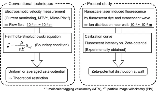
Chater 4 presents the development of a novel optical measurement technique using a fluorescent dye and the evanescent wave for inhomogeneous zeta-potential at the microchannel wall. This technique is termed nanoscale laser induced fluorescence (nano-LIF) imaging.

Figure 1.6 shows the concept of the proposed measurement technique. In conventional techniques, the wall zeta-potential is estimated from the electroosmotic velocity with the scale of 10⁻⁶ ∼ 10⁻³ m, however, the use of the Helmholtz-Smoluchowski equation restricts the measurement region to the area where the zeta-potential is uniform. On the other hand, the nano-LIF imaging focuses on the ion concentration in the vicinity of the wall related to the near-wall electric polarization with the scale of 10⁻⁹ ∼ 10⁻⁸ m. Fluorescent dye, which ion- ized in the liquid, are selected for the measurement. In the vicinity of the wall, the fluorescence ions are distributed by the electric charge at the wall, i.e., the zeta-potential. Hence, the fluorescent intensity related to the zeta-potential is detected by exciting the fluorescence only

NONUNIFORM WALL ZETA-POTENTIAL MEASURED BY

MICROCHANNEL WITH

NONUNIFORM WALL ZETA-POTENTIAL MEASURED BY

FLUORESCENCE IMAGING TECHNIQUE

by

Yutaka Kazoe

School of Integrated Design Engineering Graduate School of Science and Technology

Keio University

September 2008

Abstract

Contents

List of Tables

List of Figures

Nomenclature

Chapter 1

Introduction and Objectives

1.1 Introduction

Electrophoresis (colloid, molecule) Electroosmotic flow

1 ~ 10 nm Electrophoresis (colloid, molecule) Electroosmotic flow

1 ~ 10 nm

Microfluidic device: mixing, reaction, separation, manipulation

Control of zeta-potential

• Surface modification

• FEFC*

Driving force for liquid and sample

• Problem: Nonuniform zeta-potential

Sample dispersion by secondary flow

Control of electric field

• Switching

• Array of electrode

• Conductivity gradient

Experimental investigation of the dynamics of electroosmotic flow

• Nonuniform wall zeta-potential

• Transient flow structure

Confirming or reconstructing theory Present study

Elemental technology

Novel applications and flow control technique by controlling zeta-potential and electric field

Numerical simulation Current state

Future application

Microfluidic device: mixing, reaction, separation, manipulation

Control of zeta-potential

• Surface modification

• FEFC*

Driving force for liquid and sample

• Problem: Nonuniform zeta-potential

Sample dispersion by secondary flow

Control of electric field

• Switching

• Array of electrode

• Conductivity gradient

Experimental investigation of the dynamics of electroosmotic flow

• Nonuniform wall zeta-potential

• Transient flow structure

Confirming or reconstructing theory Present study

Elemental technology

Novel applications and flow control technique by controlling zeta-potential and electric field

Numerical simulation Current state

Future application

1.2 Literature Survey

1.2.1 Velocity Measurement of Electroosmotic Flow

1.2.2 Measurement of Wall Zeta-Potential

1.2.3 Experimental Investigation of Electroosmotic Flow with Nonuni- form Zeta-Potential

1.3 Motivation and Objectives

Development of measurement techniques

Time-resolved PTV*

Near-wall and bulk velocities

Nano-LIF*

imaging

Wall zeta-potential

Nonuniform wall zeta-potential Electroosmotic flow

*

: particle tracking velocimetry (PTV), *

: laser induced fluorescence (LIF)

*

: particle image velocimetry (PIV) Micro-PIV*

Bulk velocity

Experimental investigation

Pattern of surface modification Ion motion in flow field

• Transient flow structure

• Volumetric flow rate Steady flow structure in mixing of two solutions