九州大学学術情報リポジトリ
Kyushu University Institutional Repository
2次元規則浅水進行波と不規則海洋波
平川, 知明
https://doi.org/10.15017/1931955
出版情報:Kyushu University, 2017, 博士(工学), 課程博士 バージョン:
権利関係:
Two-Dimensional Regular Traveling Waves in Shallow Water and Irregular Ocean Waves
by
Tomoaki Hirakawa
Submitted to the Department of Energy and Environmental Engineering
in partial fulfillment of the requirements for the degree of Doctor of Philosophy
at
Kyushu University February 2018
⃝ c Kyushu University 2018. All rights reserved.
Author . . . . Department of Energy and Environmental Engineering
Certified by . . . . Makoto Okamura Associate Professor Thesis Supervisor
Accepted by . . . . Professor Kazuhide Ito
Professor Tohru Hada
Acknowledgements
Thinking back last five years, I have been influenced by many people. Throughout of my master course at Kyushu University, I often spent time with T. Makino and K. Tanaka who were studying atmospheric physics. Even writing reports were fun when I was with the wonderful friends. In the second semester of my master course, I luckily had a chance to study at Pusan National University in Korea as a member of the Campus Asia program. M. Namura, A. Akira, and M. Fukuma were also members of the program, and we shared most of the time at PNU. Short trip to Soul and graduation trip to Europe with them were great memories. From April 2015, thanks to Dr. H. Ito, I joined Green Asia program with Y. Furutani from CA program. Several months after I started my doctoral course, M. Michbata who specializes physics of cloud became a good friend of mine. We often ate dinner at a cafeteria, and he taught me about data manipulation and problems he was facing.
Some of his comments are inevitable to my work related to ocean waves. In May 2016, I got chance to visit Dr. J. Wilkening at the University of California Berkeley for about two months. He was very welcoming than I had expected, and I had firsthand experience on new research with him, which have gained my motivation to this filed of water waves. From 2017, R. Yoneda who studies nuclear fusion reactions and also a member of GA program became a good friend of mine. We went a gym together, often discussing science and our future. I would like to thank them all, including stuff of CA and GA programs.
Finally, I’m very grateful to my supervisor Dr. M. Okamura and associate pro- fessor Dr. H. Tsuji who have helped and guided me through this Ph.D. course.
Contents
1 Introduction 9
1.1 Background of regular waves . . . 9
1.2 Background of irregular ocean waves related to wave energy generation 14 1.3 The contribution of this thesis . . . 17
1.3.1 Symmetric fully-nonlinear biperiodic traveling waves . . . 17
1.3.2 Validity of KP equation . . . 18
1.3.3 Asymmetric fully- and weakly-nonlinear biperiodic traveling waves 19 1.3.4 Irregular ocean wave calculation for wave energy generations . 19 2 Symmetric Perturbation Solutions 21 2.1 Preliminary . . . 21
2.1.1 Fundamental water wave equations (fully-nonlinear equations) 21 2.1.2 Constructing symmetric solutions . . . 23
2.1.3 Normalization . . . 24
2.2 Perturbation solutions for short-crested waves . . . 25
2.2.1 Calculation procedure . . . 25
2.2.2 Validity . . . 27
2.2.3 Harmonic Resonance . . . 28
2.3 Perturbation solutions for long-crested waves . . . 31
3 KP Theory 37 3.1 Biperiodic KP solution . . . 37
3.2 Symmetric biperiodic KP solution . . . 39
3.3 Asymmetric biperiodic KP solution . . . 42
3.4 KP two-solitons . . . 43
3.4.1 Soliton resonance . . . 43
3.4.2 Modification against weak two-dimensional approximation . . 52
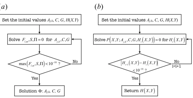
4 Symmetric Direct Numerical Solutions 53 4.1 Formulation of direct numerical solutions . . . 53
4.2 Computational method for direct numerical solutions . . . 54
4.3 Results and Discussion . . . 55
4.3.1 Fourier mode analysis . . . 57
4.3.2 Comparison of W and α for various parameters(ε, θ, D) . . . 59
4.3.3 Comparison of wave heights . . . 65
4.3.4 Correction for weak two-dimensionality approximation . . . . 69
4.3.5 Harmonic Resonance . . . 76
4.4 Conclusion . . . 76
5 Asymmetric Perturbation Solutions 81 5.1 Preliminary . . . 81
5.1.1 Constructing asymmetric solutions . . . 81
5.1.2 Normalization . . . 82
5.2 Perturbation solutions for short-crested waves . . . 84
5.2.1 Calculation procedure . . . 84
5.2.2 Results . . . 88
6 Asymmetric Direct Numerical Solutions 97 6.1 Formulation of direct numerical solutions . . . 97
6.2 Computational method for asymmetric direct numerical solutions . . 98
6.3 Results . . . 99
7 Irregular Ocean Wave 107 7.1 Data and Model . . . 107
7.2 Validation . . . 110
7.3 Result and discussions . . . 115
7.3.1 Yearly and seasonal mean wave energy transport P¯ . . . 115
7.3.2 Wave characteristics . . . 119
7.4 Conclusion . . . 123
8 Future Plan 133 8.1 Future Plan: unsteady wave motions . . . 133
A Ingredients for Computing Direct Numerical Solutions 137 A.1 Initial solution . . . 137
A.2 A Jacobian matrix for symmetric direct numerical solutions . . . 141
A.3 A Jacobian matrix for asymmetric direct numerical solutions . . . 144
A.4 The computational program . . . 146
B Perturbation Expansion 149 B.1 Mathematica script for mth order perturbation and Taylor expansions 149 C The singly periodic KP and KdV solution 153 C.1 KP and KdV solutions of Jacobian elliptic function . . . 153
Chapter 1 Introduction
1.1 Background of regular waves
Despite being common in everyday experience, many water-wave phenomena re- main difficult to understand. The main difficulty stems from nonlinear boundary conditions of the free-surface, which are not explicitly given and is to be determined by solving the governing equations. However, at the same time, water-wave phenom- ena is well endowed with mathematical methods and a fascinating subject.
Shallow water is closely related to the life of humans. Both experimental observa- tions and derivation of valid models appear to be contributed in the theory of shallow water waves, and they both suggest the importance ofnonlinearityanddispersive- ness of waves in shallow water [1, 2]. Shallow water waves are essentially nonlinear and dispersive because unless nonlinearity and dispersiveness are taken into account, solitary waves cannot maintain their profiles, rapidly falling to pieces of different sinusoidal waves. Considerable progress has been made in weakly-nonlinear (and dis- persive) theory of shallow water waves, especially interactions of shallow water waves either for solitons or periodic waves.
Korteweg-de Vries (KdV) equation is a well known weakly-nonlinear equation for one-dimensional shallow water waves, which also emerges in many physical phenom- ena [3, 4], and Kadomtsev-Petviashvili (KP) equation is a two-dimensional general- ization of the KdV equation, which has been brought to attention because of the
Figure 1-1: Photograph taken from Phares des Baleines (Whale Lighthouse) at the western point of ˆlle de Ré (Isle of Rhé), France, in the Atlantic Ocean [8].
existence of exact solutions for both solitons and periodic waves [5, 6, 7]. Account- ing for two dimensions is also important because real water waves are inherently two-dimensional rather than one-dimensional. (In this thesis, we call waves that have two-dimensional wave patterns two-dimensional waves.) Biperiodic waves are exam- ples that suggest the importance of two-dimensional effects. Biperiodic waves occur when periodic waves propagating in different directions intersect each other, or when waves reflect from a vertical wall and interact with incident waves. A photograph of relatively biperiodic waves at a coat is shown in figure 1-1.
The weakly-nonlinear theory for shallow water waves are well established in the previous century, and we are now able to know relatively accurate wave behaviors from it. However, obtaining reasonable solutions that describe fully-nonlinear fundamental water waves (i.e., direct numerical solutions) remains a challenge when waves have
very sharp crests due to the strong nonlinearity.
Studies that search for direct numerical solutions have developed enhanced cal- culation methods, and are motivated by finding limiting wave profiles [9, 10], har- monic resonances [9, 11, 12], instabilities [13, 14], the pressure exerted on a vertical wall [11, 15, 16], or the departures from weakly-nonlinear solutions [14].
The collocation method in space and time has been an effective method to calcu- late direct numerical solutions and can be implemented on computers in a straightfor- ward manner. Roberts and Schwartz (1983) [12], and Okamura (1996) [17] calculated truncated double Fourier series solutions on infinite depth by using the collocation method. However, if the waves form sharp peaks, derivatives of the free-surface displacement with respect to space become discontinuous, thus causing a severe nu- merical error. To treat this problem, Tsai and Jeng (1994) [10] invoked a kinematic condition that does not involve the derivative of the free-surface displacement η. Re- cently, Okamura (2010) [9] used Galerkin’s method to obtain large-amplitude solu- tions for an infinite depth based on truncated double Fourier series with the kinematic condition [10], thereby avoiding evaluation of any spatial derivatives of η and thus decreasing the numerical error.
As for an analytical approach, many studies have used perturbation techniques to obtain a solution to the fundamental water wave equations. This approach involves expanding solutions as a power series in the small parameterε (see, for example, [18], in which a 3rd-order perturbation solution is calculated for a finite water depth).
However, perturbation techniques often suffer from the following four limitations:
1. The radius of convergence of solutions is smaller than the maximum wave am- plitude.
2. If the fundamental mode (j, k) = (1,1) is assumed, which implies that higher Fourier modes can only be generated at higher orders, the solutions cannot represent harmonic resonant solutions consisting of higher Fourier modes of the same order with the fundamental mode.
3. If the waves form a nearly one-dimensional wave profile (long-crested waves),
the Fourier modes related to the direction perpendicular to the propagation direction slowly decrease with increasing the wave number. Such waves occur when two waves propagating in almost the same direction interact strongly with each other.
4. In shallow water, the wave width narrows and thus requires higher Fourier modes.
Using a semi-analytic approach, Roberts (1983) [12] devised an algorithm to perform the perturbation technique that enables to calculate the 27th high order perturbation solutions. Furthermore, he applied the Padé approximation to accelerate the conver- gence of the solutions. Marchant and Roberts (1987) [15] generalized this algorithm to the finite-depth case and obtained the 32nd order solutions.
Nicholls and Reitich (2006) [19] pointed out the above semi-analytic algorithms suffer from numerical instability at high order due to subtle but significant cancel- lations. They furthermore provided a new, stable high-order perturbation algorithm based on a work of Nicholls and Reitich (2005) [20] which describes that a change of variables prior to the perturbation expansion succeeds as it implicitly accounts for all significant cancellations.
As mentioned, biperiodic perturbation solutions for short-crested waves become singular when both two waves propagate in almost the same direction, which corre- sponds toθ →90◦. This is because the method presumes higher Fourier modes occur in higher orders, setting only a Fourier mode (j, k) = (1,1)for the1st order. Assum- ing 90◦−θ = O(ε), Roberts and Peregrine (1983) [21] showed a way to circumvent the problem and obtained a long-crested wave solution based on the Jacobian elliptic function, which includes higher Fourier modes even in the 1st order.
The KdV equation, obtained by Korteweg and de Vires (1895) [3], may be one of the most well known shallow water wave equation. Derivation of the KdV equation was an important benchmark because it has the particular solution as asech2 profile, which is insisted to exist by Boussinesq in 1870 and Lord Rayleigh in 1879. Jaco- bian elliptic, such as dn2, is merely a superposition of the sech2; therefore, the KdV
equation also allows dn2 as a solution, which is known as the cnoidal wave.
The KP equation is a weakly-nonlinear equation for shallow water waves and known to have biperiodic solutions involving the Riemann theta function (i.e., KP so- lutions of genus-2, hereinafter referred to as biperiodic KP solution) [5]. By assuming weak two-dimensionality, the KP equation can be derived by extending the KdV equa- tion, so that the two equations share most of their assumptions. Satsuma (1979) [22]
showed that this equation has multisoliton (N-solitons) solutions. One can find pho- tographs of soliton interactions on beaches in a paper by Ablowitz (2012) [23]. The KP equation also accepts a singly periodic solution of a Jacobian elliptic function or KP solutions of genus-1. Nakamura (1979) [7] and Dubrovin (1981) [6] proved that the Riemann theta function satisfies the KP equation, provided that the pa- rameters satisfy certain relations. The KP equation is more complex than the KdV equation in that KP solutions of genus-2 cannot be composed with a simple su- perposition of N-solitons due to two-dimensional interactions of waves. Segur and Finkel (1985) [24] presented practical ways to construct this biperiodic KP solution, gave explicit relations that solution parameters must satisfy, and conjectured that biperiodic KP solution represents typical two-dimensional periodic wave phenomena on shallow water. Akylas (1994) [25] shows an aerial photograph of real shallow wa- ter wave patterns, which supports this conjecture. One can find more photographs that look like biperiodic KP solutions in a paper by Hammack et al. (1995) [26] and Segur (2007) [27]. Motivated by this conjecture, Hammack et al. (1989) [28] and Hammack et al. (1995) [26] respectively compared symmetric and asymmetric wave patterns of biperiodic KP solution against experimental results obtained in a wa- ter pool. The biperiodic KP solution describes the measured waves with reasonable accuracy, even beyond the putative range of the KP theory.
The KP and KdV solutions, which involve Jacobian elliptic functions, and the biperiodic KP solutions all approach solitons as the wavelength approaches infinity.
Miles (1977) [29] derived a theory for interactions of solitons, finding the resonant interaction regime, that is equivalent to the KP theory; furthermore, he [30] first associated this resonant interaction with the Mach reflection. By comparing the KP
soliton with the KdV soliton, Yeh et al. (2010) [31] and Li et al. (2010) [32] clarified and corrected a deficiency that the KP soliton becomes unphysical when two such solitons propagate in significantly different directions. In addition, the corrected Miles theory and KP theory agree more strongly with numerical [33, 34] and experimental results of solitons [31], although this correction has yet to be applied to KP periodic solutions.
Comparing numerical solutions to the KP equation and the second-order funda- mental water wave equation obtained by Bryant (1982) [14] suggests that the former solutions (biperiodic KP solutions) differ significantly from the latter ones in both wave height and wave frequency for large angles between the propagation directions of the two incident waves. By using biperiodic KP solution and direct numerical solu- tions to the fully-nonlinear fundamental water wave equations, we may more precisely understand how the accuracy of the biperiodic KP solution varies with increasing wave height, interaction angle, and water depth.
1.2 Background of irregular ocean waves related to wave energy generation
The oil crises of 1973 and 1979 caused the Japanese economy to record negative growth rates for the first time in its post-war history and induced a major change in Japan’s national energy policy. The new policy, which involves greater government involvement in oil and other energy markets, included active promotion of nuclear power [35], which is favorable for a resource-poor but technology-rich nation. How- ever, after three decades, the Japanese government abruptly changed its energy policy in the wake of the Fukushima nuclear accident of March 11, 2011, the strong public opposition to nuclear power. The nuclear crisis, together with the Kyoto Protocol 2020 target of reducing carbon dioxide, posed a serious challenge to the nation’s economy and its energy security; however, following the recent adoption of the Paris Agreement at the 21st session of the Conference of the Parties (COP21), the Japanese
government set an ambitious target to reduce greenhouse gas emissions to 26% below 2013 levels in 2030 and increase the share of renewable energy from 12% in 2016 to 22%-24% by 2030 [36]. While acknowledging the difficulty for renewables to take up nuclear energy’s share in near future, the promotion of renewable energy technology is one of the key policies for Japan’s stable future energy structure.
As a part of the reconstruction and recovery of Fukushima Prefecture in the To- hoku area, the Japanese government implemented a national project named “Fukushima Innovation Coast Framework," which aims to turn the whole of Fukushima Prefecture into a base for creating a pioneering model of a future new energy-oriented society by supporting new technologies and industries. Wave energy has been drawing attention in Japan because the nation is surrounded by the sixth largest exclusive economic zone in the world, and an abundance of wave energy is available. Recently, a wave energy facility was deployed at Kuji City in Iwate Prefecture on November 7, 2016, as a part of the Next-generation Energies for Tohoku Recovery Project, which takes ad- vantage of the strengths of universities and research institutions. In addition, together with Mitsui Engineering and Shipbuilding, Ocean Power Technologies deployed their PowerBuoy technology off the north coast of Kouzu Island in Tokyo Prefecture on May 10, 2017.
Countries facing the North Sea, the Atlantic Ocean and the Southern Pacific Ocean are well endowed with wave energy resources [37], and many research and development projects are under way in these countries [38]. In Japan, the first wave energy resource assessments were performed by Maeda and Kinoshita (1979) [39], stimulated by the oil crises. Most of the long-term wave data available at that time consisted of significant wave height H1/3 (m) and wave period T1/3 (s), which were visually estimated from ships [40]. Maeda and Kinoshita (1979) calculated the distribution of mean wave energy transportP¯(kW/m) around Japan from 1954 to 1963, using visually estimated wave data and applying a Pierson-Moskowitz spectrum and an approximation of the wave energy transport P (kW/m):
P =
∫ ∞
0
∫ ∞
0
αH1/3T1/3p(H1/3, T1/3)dH1/3dT1/3, (1.1)
where α = 0.55, and p(H1/3, T1/3) describes the probability density function. The line over variables, such as P¯, indicates the mean value of the variable in this study.
For Kyushu, which is the southernmost and third largest of Japan’s four main islands, the results showed that P¯ = 11.57 in the east, ranging a latitude of 30◦-35◦ and a longitude of 130◦-135◦, and P¯= 9.91in the west, ranging a latitude of 30◦-35◦ and a longitude of 125◦-130◦. Maeda et al. (1981) [41] also obtained P¯ = 12.7for the east region and P¯ = 11.0for the west region from 1954 to 1963, using (1.1) withα= 0.57 based on the JONSWAP spectrum together with visually estimated wave data.
Applying the zero-up-crossing (zero-crossing) method, most of the wave data mea- sured by an ultra sonic wave gauge (USW) have been collected since the 1970s. Tabata et al. (1980) [42] obtained a mean wave energy transport value of P¯ = 7.28 for southeast of Kyushu and P¯ = 0.623 southwest of Kyushu for 1975 to 1978, using zero-crossing data and an approximation
P = 0.5H1/32 T, (1.2)
where T (s) is the mean zero-crossing wave period. They concluded that previous results [39, 41] overestimated the mean wave energy transport P¯ due to the use of inaccurate visually estimated wave data. Takahashi et al. (1989) [43] obtained P¯ = 6.7 southeast of Kyushu and P¯ = 1.6 southwest of Kyushu for 1970 to 1984, using an approximation
P¯ = 1.35µσ1/3H¯1/3T¯1/3, (1.3) where σ1/3 is the standard deviation of the significant wave height H1/3, and µ is a parameter that takes µ = 1.0 for Japan Sea coasts and µ = 0.5 for Pacific Ocean coasts. Directions and positions of the mean wave energy transport P¯ propagating from the southeast and southwest toward Kyushu described by Tabata et al. (1980) and Takahashi et al. (1989) are depicted in figure 7-1. Takahashi et al. (1989) also studied the joint distribution of H1/3 and T1/3 around Japan; however the wave direction and directional spectrum were not discussed, though they insisted on the necessity analyzing wave direction and directional spectrum. In the early studies,
spatial resolutions of analyses were coarse, because of the limited number of site measurements, thus comprehensive wave characteristics have yet to be performed.
Recently, a wave energy assessment was performed for Japan between 1994 and 2014 using WaveWatchIII model with 1 km grid cells [44]. The mean wave energy transport 30 km off Japanese coasts was estimated as P¯ = 7.35. However, comprehensive analyses of waves around Kyushu were not discussed.
1.3 The contribution of this thesis
As mentioned above, although we can know wave behaviors relatively accurately from the weakly-nonlinear theories, obtaining direct numerical solutions from fully- nonlinear equations remains a challenge when wave crests are large. There have been few studies that go beyond weakly-nonlinear theories of two-dimensional shallow water waves [34]. No study has succeeded to calculate large two-dimensional waves in shallow water.
At the most basic level, this thesis addresses fully- and weakly-nonlinear biperi- odic traveling waves by using either analytical or computational method. The last chapter is the exception which studies irregular ocean waves for wave energy generation.
1.3.1 Symmetric fully-nonlinear biperiodic traveling waves
For one-dimensional wave case, there is a computational method to calculate lim- iting waves with very high accuracy, using the conformal mapping [45]. For two- dimensional wave cases, as mentioned in section 1.1, perturbation methods are of- ten used. However, large amplitude shallow water waves cannot be calculated by the usual perturbation method. The extended perturbation method of Roberts and Peregrin (1983) [21] may calculate shallow water waves more accurately, though the method still assumes waves with small amplitudes. The computational method de- veloped by Okamura (2010) [9] is remarkable in that it can calculate even two- dimensional large amplitude waves with high accuracy because the wave height is
not Fourier expanded and do not suffer from the small radius of convergence.
In chapter 2, we review the perturbation solutions, including interesting resonance phenomena. In chapter 4, we calculate symmetric direct numerical solutions to fully- nonlinear equation, using Okamura’s method as a basis for the computation. This method enables us to obtain solutions with relatively large amplitude shallow water waves, which is the highlight of this thesis.
1.3.2 Validity of KP equation
Boussinesq equations, Benney-Luke equation, and the KP equation are weakly- nonlinear equations that describe shallow water waves. They all assume the weak nonlinearity and weak dispersivity and take up to the quadratic nonlinearity into ac- count. Furthermore, the KP equation can be obtained by assuming weakly-nonlinear, weakly-dispersive, weakly-two-dimensional waves from the fully-nonlinear equations (fundamental water wave equations). Even though the KP equation is based on many approximations, why is it important? Theoretically, one can get higher non- linear biperiodic solutions than these weakly-nonlinear equations, setting numbers of different Fourier modes at the 1st order of the solution. However, in this way, it is too costly to calculate high orders. The KP solution has the exact biperiodic solu- tion, which has been studied well, whereas Boussinesq equations and Benney-Luke equation don’t have ones.
Biperiodic KP solutions were confirmed to exist by experiments [28, 26] and obser- vations of wave patterns at coasts [25, 26]. However, there are few studies that address validities of weakly-nonlinear solutions by comparing them with fully-nonlinear solu- tions [34, 14, 33]. In chapter 3, we review KP solutions mostly based on work of Segur and Finkel (1985) [24] and Miles (1977) [46, 29]. In chapter 4, to clarify how the ac- curacy of the biperiodic KP solution is affected when some of the KP approximations are not satisfied, we compare the fully- and weakly-nonlinear periodic traveling waves of various wave amplitudes, wave depths, and interaction angles.
Furthermore, to remedy the weak two-dimensionality approximation, we apply the correction of Yeh et al. (2010) [31] to the biperiodic KP solution, which substantially
improves the solution accuracy and results in wave profiles that are indistinguishable from most other cases.
1.3.3 Asymmetric fully- and weakly-nonlinear biperiodic trav- eling waves
To the best of my knowledge, previous studies related to both short-crested and long-crested waves are all assumed as symmetric waves: interactions of two waves which have the same wave amplitude and frequency. Although the KP solution can express asymmetric waves, we still don’t know if there is asymmetric biperiodic travel- ing waves for fully-nonlinear equations. First, we construct asymmetric perturbation solutions in chapter 5. Based on the formulation, we proceed to calculate asymmet- ric direct numerical solutions to the fully-nonlinear equation, generalizing the method used in chapter 4. Figure 1-2 shows a schematic of different approaches for symmetric and asymmetric biperiodic traveling waves.
1.3.4 Irregular ocean wave calculation for wave energy gen- erations
It is important to understand wave characteristics, including wave direction and directional spectrum to assess the eligibility of wave energy for power generation [43].
What seems to be lacking to assess waves around Japan is detailed scrutiny of wave characteristics. Accordingly, we aim to present comprehensive analyses of statistics of wave characteristics around Kyushu using a high-resolution numerical model in chapter 7.
Biperiodic Traveling Waves Analytical Numerical
Fully-nonlinear equations (Fundamental water wave equations)
The KP equation
Symmetric direct solutions in shallow water
for short-crested waves
Symmetric mth order perturbation
solutions
Asymmetric direct solutions in shallow water
Asymmetric mth order perturbation
solutions
for long-crested waves
Biperiodic KP solutions
Introduce small parameters
Symmetric mth order perturbation
solutions
Figure 1-2: Schematic showing different approaches for symmetric and asymmetric biperiodic traveling waves. Chapter 4 and chapter 5 study asymmetric solutions described with red lines at right and left.
Chapter 2
Symmetric Perturbation Solutions
In this chapter, we review symmetric perturbation solutions including short- crested and long-crested waves.
2.1 Preliminary
2.1.1 Fundamental water wave equations (fully-nonlinear equa- tions)
We use a Cartesian coordinate system(x, y, z)in whichxand yare the horizontal coordinates, andz increases upward. We consider the three-dimensional irrotational flow of an inviscid and incompressible fluid bounded below at flat bottomz =−hand above by a free-surfacez =η(x, y, t)as shown in figure 2-1. Since the flow is assumed to be irrotational, a velocity potentialϕ(x, y, z, t)exists such thatv=∇ϕ wherevis the fluid velocity, and∇= (∂/∂x, ∂/∂y, ∂/∂z)is the vector differential operator. The fully-nonlinear water wave equations that govern η(x, y, t) and ϕ(x, y, z, t) consist of Laplace’s equation
∆ϕ= 0 for −h≤z ≤η(x, y, t), (2.1) with the bottom condition
ϕz = 0 on z =−h, (2.2)
Figure 2-1: Schematic of variables.
the dynamic boundary condition ρ(x, y, z, t) = ϕt+β+1
2∇ϕ· ∇ϕ+gz = 0 on z =η(x, y, t), (2.3) and the kinematic boundary condition
D
Dtρ(x, y, z, t) = 0 on z =η(x, y, t), (2.4) where ∆ = ∇ · ∇ is the Laplacian, subscripts denote partial derivatives, g is the acceleration due to gravity in the negative z direction, β is an arbitrary constant that is necessary to determine the mean water depth, and D/Dt = (∂/∂t+∇ϕ· ∇) is the Lagrangian derivative operator. (2.4) is obtained by applying D/Dt to (2.3), describing that there is no change of the pressure on a fluid parcel at the free-surface with time, as it follow along its trajectory [9, 10, 47]. Since it is not obvious that (2.4) can be replaced with the usual kinematic condition: Df /Dt= 0 wheref(x, y, z, t) = z −η(x, y, t) = 0 on the free-surface z = η, we show the derivation of (2.4) in the following. Noting that the pressure on the free-surface is constant along the free- surface, we have
0 = D2
D2tρ(x, y, η, t) =
{Dρ
Dt +ρz(ηt+∇2ϕ· ∇2η−ϕz)
}
z=η(x,y,t)
, (2.5) where D2/D2t = (∂/∂t+∇2ϕ· ∇2) and ∇2 = (∂/∂x, ∂/∂y). (2.5) means (2.4) is equivalent to the usual kinematic condition ηt+∇2ϕ · ∇2η −ϕz = 0 on the free-
surface z =η when ρz ̸= 0.
2.1.2 Constructing symmetric solutions
We start from considering superposition of two wave trains, which satisfy Laplace’s equation (2.1).
ϕ(x, y, z, t) =
a1r(z;µ1, ν1) sinψ1 +a2r(z;µ2, ν2) sinψ2
, ψj =µjx+νjy−ωjt, j = 1,2. (2.6)
where
r(z;µj, νj) = cosh[√µj2 +νj2(z+h)] cosh(√µj2+νj2h)
. The condition for symmetric waves is
(µ1, ν1, ω1) = (µ2,−ν2, ω2), a1 =a2. (2.7) Let us rewrite as (µ1, ν1, ω1) = (µ2,−ν2, ω2) = (κx, κy, ω) and a1 = a2 = a. (2.7) describes
ϕ=ar(z;κx, κy) sin (κxx−ωt) cos (κyy). (2.8) Because Laplace’s equation is linear, superpositions of such waves are also accepted as solutions:
ϕ(x, y, z, t) =
∑∞ j=1
∑∞ k=0
aj,kr(z;jκx, kκy) sin [j(κxx−ωt)] cos (kκyy). (2.9)
2.1.3 Normalization
We introduce the following dimensionless quantities and moving coordinate sys- tem, assuming waves propagate in the x direction without change in the form:
X =κxx−ωt, Y =κyy, Z =κz, D=κh, G= κ
ω2g, C = κ2 ω2β, H(X, Y) =κη(x, y, t), Ψ (X, Y, Z) = κ2
ωϕ, Φ (X, Y, Z) = κ2 ω
{
ϕ− ω κx
(
x− ω κxt
)}
. (2.10) whereκis the wavenumber of the incident wave,ω is the wave frequency, and defining (p, q) = (sinθ,cosθ),(κx, κy) = (κp, κq)is the wavenumber vector of biperiodic waves.
In this paper, we will refer to θ as “the interaction angle”. The solutionΨ becomes Ψ (X, Y, Z) =
∑∞ j=1
∑∞ k=0
Aj,kRj,ksin (jX) cos (kY), Rj,k(Z) = cosh [αj,k(Z +D)]
cosh (αj,kZ) =r(z;jκp, kκq),
(2.11)
where αj,k =√
j2p2+k2q2.
The normalization of Φ seems complex, but this makes the boundary conditions simpler. ΦandΨare respectively considered as the velocity potential with and with- out the mean flow, which occurs due to the Galilean transform. Laplace’s equation, dynamic condition, and kinematic condition based on Φare
L=p2ΦXX +q2ΦY Y + ΦZZ = 0 as −D≤Z ≤H, (2.12) P = 1
2
(
p2Φ2X +q2Φ2Y + Φ2Z−p−2)+GZ+C = 0 on Z =H, (2.13) Q=p2ΦX(p2ΦXΦXX+q2ΦYΦXY + ΦZΦXZ)
+q2ΦY (p2ΦXΦXY +q2ΦYΦY Y + ΦZΦY Z)
+ ΦZ(p2ΦXΦXZ +q2ΦYΦZY + ΦZΦZZ +G)= 0 on Z =H. (2.14)
Laplace’s equation, dynamic condition, and kinematic condition based on Ψare L=p2ΨXX +q2ΨY Y + ΨZZ = 0 as −D≤Z ≤H, (2.15) P = 1
2
(
p2Ψ2X +q2Ψ2Y + Ψ2Z−2ΨX)+GZ+C = 0 on Z =H, (2.16) Q= (p2ΨX −1) (p2ΨXΨXX +q2ΨYΨXY + ΨZΨXZ−ΨXX)
+q2ΨY (p2ΨXΨXY +q2ΨYΨY Y + ΨZΨY Z−ΨXY)
+ ΨZ(G+p2ΨXΨXZ+q2ΨYΨZY + ΨZΨZZ −ΨXZ)= 0 on Z =H. (2.17)
2.2 Perturbation solutions for short-crested waves
2.2.1 Calculation procedure
The perturbation methods are useful to reduce nonlinear differential equations to linear differential equations. The usual procedure of perturbation methods is to substitute suitable expansions in powers of a small parameter ε into the differential equations, and then grouping the differential equation by powers of ε, we get an infinite system of linearized equations which may be successively solved. We review how to successively solve the fully-nonlinear equations (2.15), (2.16), (2.17), and study harmonic resonances.
We first introduce the small parameterε, which will be eventually replaced with the 1st order wave amplitudeA(1)1,1. We expand the boundary conditions (2.16) and (2.17) in power of ε as
P (X, Y, H) =
∑∞ m=0
εmP(m)(X, Y), Q(X, Y, H) =
∑∞ m=0
εmQ(m)(X, Y).
Here, P(n) and Q(n) no longer depend on the free-surface displacement H because variables Ψ and its all derivatives are also Taylor expanded. For example, variables
are expanded as G=
∑∞ m=0
εmG(m), C =
∑∞ m=1
εmC(m), Ψ(X, Y, Z) =
∑∞ m=1
εmΨ(m), H(X, Y) =
∑∞ m=1
εmH(m), (2.18)
where
Ψ(m)(X, Y, Z) =
∑∞ j=1
∑∞ k=0
A(m)j,k Rj,ksin (jX) cos (kY), (2.19) H(m)(X, Y) =
∑∞ j=1
∑∞ k=0
Bj,k(m)cos (jX) cos (kY). (2.20)
Ψ on the free-surface is expanded as
Ψ (X, Y, H) =
∑∞ n=0
1 n!
∑∞
j=1
εjH(j)
n∑∞ i=1
εi∂nΨ(i)
∂Zn
Z=0
,
which corresponds to equation (21) in Hsu (1979) [18]. The 1st order dynamic and kinematic conditions become
Q(1) = Ψ(1)XX+G(0)Ψ(1)Z = 0, (2.21) P(1) =C(1)+G(0)H(1)−Ψ(1)X = 0. (2.22) The mth order dynamic and kinematic conditions become
Q(m) = Ψ(m)XX+G(0)Ψ(m)Z +G(m−1)Ψ(1)Z −f(m) = 0, (2.23) P(m) =C(m)+G(0)H(m)−Ψ(m)X −g(m)= 0. (2.24) where f(m), g(m) are nonlinear terms, which consist of variables of lower orders. Dur- ing the calculation, we need to be careful about the non-secularity condition, which sometimes tell us a nontrivial condition to set. In this case, we can always avoid secular terms by choosing G(m−1) as
G(m−1) = F1,1
[
f(m)] F1,1
[
Ψ(1)Z ], (2.25)
where Fµ,ν is defined as
Fµ,ν[f(X, Y)] =
4 π2
∫ π
0
∫ π
0
f(X, Y) sin (µX) sin (νY)dXdY µ̸= 0, ν̸= 0 2
π2
∫ π
0
∫ π
0
f(X, Y) sin (µX)dXdY µ̸= 0, ν= 0 2
π2
∫ π
0
∫ π
0
f(X, Y) sin (νY)dXdY µ= 0, ν̸= 0 .
(2.26) Using the kinematic condition (2.23), A(m)j,k can be successively calculated as
A(m)j,k = Fj,k
[
f(m)+G(m−1)Ψ(1)Z ]
G(0)αj,ktanh (αj,kD)−j2. (2.27) SubstitutingA(m)j,k into the dynamic condition (2.24), Bj,k(m) can be successively calcu- lated as
Bj,k(m) = F˜j,k
[
g(m)+ Ψ(m)X ]
G(0) , (2.28)
where F˜µ,ν is defined as
F˜µ,ν[f(X, Y)] =
4 π2
∫ π
0
∫ π
0
f(X, Y) cos (µX) cos (νY)dXdY µ̸= 0, ν ̸= 0 2
π2
∫ π
0
∫ π
0
f(X, Y) cos (µX)dXdY µ= 0, ν ̸= 0 2
π2
∫ π
0
∫ π
0
f(X, Y) cos (νY)dXdY µ̸= 0, ν = 0 1
π2
∫ π
0
∫ π
0
f(X, Y)dXdY µ= 0, ν = 0 .
(2.29) C(m) is determined asC(m) = ˜F0,0
[
g(m)].
2.2.2 Validity
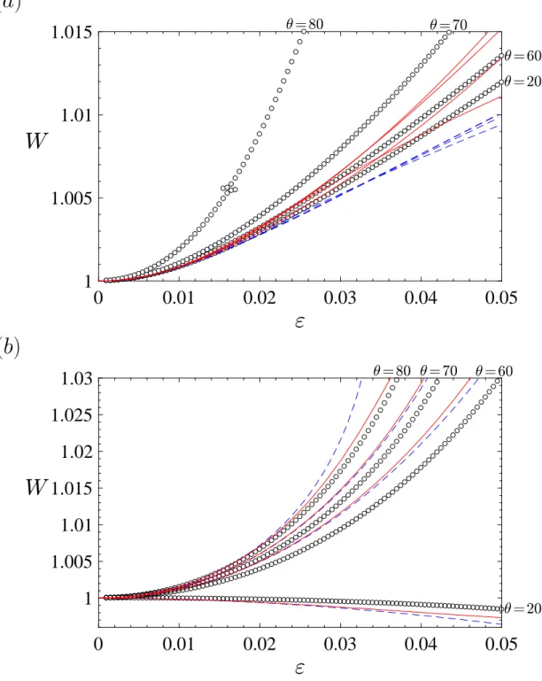
Figure 2-2 compares normalized wave speed W between the 3rd order, 6th order solutions, and direct numerical solutions which will be calculated in chapter 4, over the nonlinear parameter ε and various interaction angles θ = 20◦,60◦,70◦,80◦. We
define the nonlinear parameter ε as εD−H
(π 2,π
2
)
+H(π,0) = 0. (2.30)
This figure shows that perturbation solutions are relatively accurate for the deep water wave case than the shallow water wave case. This is because Fourier modes with large wavenumbers become significant in shallower water.
2.2.3 Harmonic Resonance
For short-crested waves, setting the wave numbers (j, k) = (1,1) for the linear solution an higher harmonic becomes infinite when a certain set of (D, θ) satisfies a relation:
αj,ktanh (αj,kD) = j2tanh (D), (2.31) which implies that the higher harmonic is resonated with the linear wave of (j, k) = (1,1), that is the order of the higher harmonic is inappropriate. This condition can be obtained from the kinematic condition (2.23), which unknown terms become
{
Ψ(m)XX+G(0)Ψ(m)Z }
Z=0 ={Aj,k(−j2Rj,k+G(0)Rj,k,1)sin (jX) cos (kY)}
Z=0, where Rj,k,n = ∂n
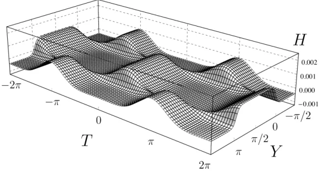
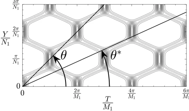
∂ZnRj,k, and G(0) = coth (α1,1D) if the 1st order solution is set to (j, k) = (1,1). When the unknown terms become zero for a combination of the depth D and the angle θ, Aj,k cannot be determined by comparing coefficients with those of corresponding trigonometric functions which consist of nonlinear couplings. This condition is the same as (2.31), which describes that the amplitudeAj,k grows infinity for infinitely large value of time. For (j, k) = (1,1), the same error always occur, no matter what the water depth D and angle are. This tells us a condition that the system should universally satisfy. Such an error can be circumvented by expanding the frequencies Ω for each order m. Figure 2-3 shows bifurcation diagrams of A(4)2,4, A(5)3,5, and A(6)4,6 over the interaction angle θ for A(1)1,1 = 0.001. Figures 2-4 and 2-5 respectively show wave profiles forD=π/50, ε= 10−4 and their contour plots. The
(a)
0 0.01 0.02 0.03 0.04 0.05
1 1.005 1.01 1.015
(b)
0 0.01 0.02 0.03 0.04 0.05
1 1.005 1.01 1.015 1.02 1.025 1.03
Figure 2-2: The 3rd order solution, – –; 6th order solution, —; direct numerical solutions, ◦. (a), D = 2π/50: the shallow water wave case; (b), D = 2π: the deep water wave case.
(a)
(b)
(c)
Figure 2-3: Bifurcation diagrams for A(1)1,1 = 0.001, (a) A(4)2,4, (b) A(5)3,5, and (c) A(6)4,6. Red lines in the fronts of figures are results for the depthD=π/50(100 times smaller than the wave length 2π).
depth D and interaction angle θ of (a) and (c) in the figures are almost equivalent to the harmonic resonance condition of (j, k) = (3,5) and (2,4), respectively. For example, A(4)2,4 can be obtained as
A(4)2,4 = A(1)1,1 192 (R2,4,1−4)
−24A(1)1,1A(2)2,2(−2p2R1,1,2−3R2,2,2+ 8p4+ 14p2+ 8)
−A(1)31,1 (3R1,1,2(−R1,1,2+ 12p2−1) +R1,4,4+ 36p4−36p2+ 5) +48A(3)1,3(−R1,1,2+ 3R1,3,1−R1,3,2+ 10p2−11)
−48A(3)3,3(−3R1,1,2+R3,3,2+ 24p2−24)
,
where Rj,k,n = ∂Z∂nnRj,k. A(5)3,5 can be obtained as
A(5)3,5 = 1
2048 (9−R3,5,1)
256A(1)1,1
A(2)22,2 (−(2p2+ 5)R2,2,2+ 3R1,1,2 + 8 (p2+ 5)p2−3) +2A(4)2,4(2R1,1,2−8R2,4,1+R2,4,2−20p2+ 22)
+2A(4)4,4(−4R1,1,2−10R4,4,1+R4,4,2 + 48p2−20)
+16A(1)31,1 A(2)2,2
R1,1,2(−11R2,2,2+ 160p2−68) + 4R21,1,2+R2,2,4 +2 (4 (4p2 + 1)R2,2,2+R1,4,4+ 88p4−68p2+ 3)
−64A(1)21,1
A(3)1,3
8 (3p2−4)R1,3,1+ 2R1,1,2(R1,3,1 −2p2+ 7) +9R1,3,2 −R1,3,3+ 6p4−20
−2A(3)3,3(−6p2R1,1,2−11R3,3,2+ 24p4 + 102p2+ 45)
+A(1)51,1
4R1,1,2(R1,1,2(R1,1,2+ 12p2 −6) + 6 (2p2(p2+ 6)−3))
−9R1,4,4+ 48 (4p2−7)p2+ 101
−512A(2)2,2A(3)1,3(6R1,3,1−2R1,3,2−R2,2,2+ 28p2−28)
.
A(4)2,4is involved inA(5)3,5. The number of bifurcations increases as the order of amplitude increases because higher order amplitudes usually involve lower order amplitudes, which sometimes themselves involve harmonic resonances.
2.3 Perturbation solutions for long-crested waves
By the usual perturbation method for short-crested waves, even for waves in deep water, long-crested waves cannot be calculated because of zero-divizors at θ →90◦.
(a)
(b)
(c)
Figure 2-4: Wave profiles for D = π/50, ε = 10−4, and (a), θ = 86; (b), θ =
(a)
(b)
(c)
Figure 2-5: Wave profiles for D = π/50, ε = 10−4, and (a), θ = 86; (b), θ = 85.56905136;(c),θ = 87.918345.
This is because the usual perturbation expansion implicitly assumes that higher Fourier modes have to be small, which contradicts the case of long-crested waves.
Roberts and Peregrine (1983) [21] analytically calculated long-crested waves, devel- oping the method of Whitham (1976) [48]. Their solutions involve Jacobian elliptic function sn at the 3rd order, and the solutions match onto the short-crested waves on the one hand and onto the well-known two-dimensional progressive waves on the other hand. In the following, we simply generalize their work of long-crested waves in deep water to finite water waves and confirm a wave profile of long-crested waves in deep water.
To calculate long-crested waves, we expand p2 = sin2θ and q2 = cos2θ as p2 = 1− ∑∞
n=1
εnγ(n), q2 =
∑∞ n=1
εnγ(n), (2.32)
where γ is the aspect-ratio, and Roberts and Peregrine [21] found that γ(2n−1) = 0 (n = 1,2,3, ...) for appropriate scaling. This scaling means that solutions up to 2nd order are Stokes waves propagating in the X direction. As Whitham (1976) [48] showed, Φ(m)XX can be eliminated from the kinematic conditionby using Laplace’s equation expanded on Z = 0:
L(m) =γ(1)(Ψ(mY Y−1)−ΨXX(m−1))+ Ψ(m)XX+ Ψ(m)ZZ +w(m) = 0, (2.33) where w(m) is the nonlinear term constituted from lower orders variables. Then, we have decoupled nonlinear PDE.
L(m)−Q(m)=
Ψ(m)ZZ −G(0)Ψ(m)Z = 0 m = 1
Ψ(m)ZZ −G(0)Ψ(m)Z
+γ(1)(Ψ(mY Y−1)−Ψ(mXX−1))+w(m)+f(m)−G(m−1)Ψ(1)Z = 0 m ≥2 .
(2.34) The forcing in (2.34) contains components of homogeneous solution which force secu- lar terms intoΨ(m). The non-secularity condition is a second-order differential equa-
![Figure 1-1: Photograph taken from Phares des Baleines (Whale Lighthouse) at the western point of ˆlle de Ré (Isle of Rhé), France, in the Atlantic Ocean [8].](https://thumb-ap.123doks.com/thumbv2/123deta/9915100.1917958/11.918.143.778.108.588/figure-photograph-phares-baleines-lighthouse-western-france-atlantic.webp)