Study on high field side injection of X-modefor EBW conversion in QUEST

(1)

九州大学学術情報リポジトリ

Kyushu University Institutional Repository

Study on high field side injection of X-mode for EBW conversion in QUEST

ハテム, オマ, アミン, モスタファ, エルセラフィ

https://doi.org/10.15017/2534468

出版情報：九州大学, 2019, 博士（理学）, 課程博士バージョン：

権利関係：

(2)

Doctoral Thesis

Study on high field side injection of X- mode for EBW conversion in QUEST

ASEM, IGSES, Kyushu University

Hatem Elserafy

(3)

Acknowledgement

First and foremost, I would like to attribute this work to Prof. Kazuaki Hanada as he not only had an essential role in the completion of said work, but he also had the patience and resilience to teach and pass on his indispensable knowledge to myself as well as my colleagues. Prof. Hanada’s instructions and innovative teaching techniques have never failed to inspire me. Conducting experiments alongside Prof. Hanada, watching him in action while listening to him giving me technical advice on how to deal with plasma physics has been a major highlight in my career. In addition, his support was not only limited to my doctoral studies but also to my career after graduation, to my mental and physical wellbeing, and to my life outside of the lab. Not to mention, he was very open to my pursuit of extracurricular activities alongside studying and he encouraged me to have a healthy balanced life. Not to mention, his hilarious sense of humor was very much enjoyed during parties and celebrations. Despite this man’s name speaking for itself, I cannot help but acknowledge his greatness in this modest thesis.

To Prof Kiichi Hamamoto, I would like to thank you for the support that you have given me throughout the five years of masters and doctoral studies. The gratitude I have for the amount of knowledge you have taught me is far more than words can describe. You have provided me with different opportunities to engage with the scientific and the industrial fields and most of all, you have always respected and encouraged me. I am forever grateful to what you have given me.

I am particularly grateful to Dr. Takumi Onchi, Prof. Hiroshi Idei, Prof. Masayuki Ono, Prof.

Makoto Hasegawa, Prof. Kazuo Nakamura, Dr. Nicola Bertelli, Dr. Ryuya Ikezoe, Dr. Kengoh Kuroda and Dr. Arsieny Kuzmin. Without their expertise in the field and their tremendous support, this work would not have been successful. I am honored to have shared the same facilities with such giants and for borrowing their time and wisdom ever so frequently.

Further gratitude is directed towards my colleagues, Dr. Ryota Yoneda, Mr. Shinichiro Kojima, Mr. Takahiro Murakami, Mr. Masaharu Fukuyama and Ms. Miu Yunoki. Their academic support as well as their shared memories outside the lab are unforgettable. Special thanks are due towards Dr. Yoneda and Mr. Kojima for their constant support outside of the lab to help me deal with my everyday problems and for being excellent life-coaches to me.

In addition, I would like to thank the administrative staff in general. Special thanks to Mrs. Kaori Yamaguchi for her bureaucratic support and to Mrs. Azusa Kawamura for bridging my language gap and helping me with my job hunting.

In addition, I would like to thank every member of QUEST team. It was an honor to share QUEST with you all and to collaborate with you.

Last but by no means least, to my family, I would like to gift them my doctoral thesis in hopes to make them feel proud. To my father, Omar Elserafy, my mother, Hanan Eissa, and my sister, Dina Elserafy, I am forever indebted to you for every single accomplishment I make in my life. My world is so much easier than it should be, just because I have my family as my backbone to protect me and help me move forward.

(4)

i

Abstract

Electron Bernstein Wave (EBW) is a candidate for overcoming the density limit for RF induced plasmas in the electron cyclotron range of frequency, although EBW, an electrostatic wave, can only be created inside of the plasma via mode conversion. Several mode conversion scenarios exist including Ordinary-Extraordinary-Bernstein (O-X-B) wave conversion from low field side (LFS), direct X-B conversion from LFS, and X-B conversion from high field side (HFS). LFS launch has been conducted in QUEST with low efficiency and inability to surpass the cutoff limit using 8.2 GHz RF injection. HFS injection of X-mode to EBW mode is expected to have higher conversion efficiency, so it was the target of this work.

In the Section 1, introduction and necessity of nuclear fusion development are described. It is clearly indicated that to satisfy both electric power production to progress mankind and mitigation of climate change, new technologies such as nuclear fusion are indispensable. Tokamak is the most promising way to realize a fusion power plant on the earth and several kinds of alternative ways are introduced. Spherical tokamak (ST) has a possibility to achieve cost-effective fusion power plant, but development of non-inductive way to produce plasma current that needs to make a plasma equilibrium in tokamak type of magnetic fusion devices is the most crucial issue. RF current drive has been developed for overcoming the issue and the remaining is to produce higher density plasma with only RF. After that, other techniques such as neutral beam injection and so on are available.

In the Section 2, basic physics for wave propagation and absorption in plasma are described.

Several scenarios to excite electron Bernstein wave (EBW) are specifically introduced. The merit and demerit are compared and the reason why the X mode injection from high field side (HFS) should be selected is clarified in the view of theoretical basis consideration.

In the section 3, two important codes for quantitative estimation of wave absorption and driving plasma current are introduced. EFIT was used to analyze the magnetic surface in QUEST, then calculate the magnetic reconstruction as an input for GENRAY ray tracing code that can estimate wave absorption and driven current. According to GENRAY’s simulations, inputting further density than 1.5×10¹⁸m^-3 would lead to 𝜔_𝑝𝑒 (plasma cut-off) layer development enough to bend the X-mode ray out of UHR’s access. GENRAY also provided output that the injected ray has to be tilted above or below the mid-plane if EBWCD was of interest, such that above the mid-plane would create a counterclockwise Ip and below the mid-plane would create a clockwise Ip in the condition of present magnetic surface in QUEST. In conclusion, HFS injection of X-mode with an injection tilt angle is expected to drive EBWCD, therefore a tilt or a shift is to be considered in injection system design, which is to be discussed in the next section.

In the Section 4, the HFS injection system design is discussed. a waveguide-based RF transmission line from LFS to HFS for 8.2 GHz which is equipped in QUEST is proposed. This system has the advantage of working in any frequency range as well as not suffering any reflective losses from reflecting mirrors that were used in the other devices. The transmitted RF should be emitted by a simple open-ended waveguide. The dispersion and non-desired RF absorption were accounted for, showing no more than 7% losses in the plasma of 50eV electron temperature. To summarize, the HFS injection system could be designed, based on optimizing wave transmission and minimizing undesired RF absorption in the present specification of QUEST.

In the section 5, the experimental results are denoted. The experiment has been executed by using only toroidal magnetic field to simply investigate the EBW mode conversion. The electron temperature using Langmuir probe in the HFS case was at an average of 4 eV, while in the LFS case it was about 2 eV. Moreover, the brightness of the fast camera images in the case of HFS launch is significantly higher than those in LFS launch. An interferometer was used to measure line-averaged density and it finds that the position of UHR estimated by the measured density corresponds to the brightest position in the fast camera images. This clearly indicates that EBW could be excited in the plasma and deposited via collisional damping as predicted by GENRAY calculation. Higher density and temperature in HFS launch suggests having better mode

(5)

ii

conversion efficiency than that in LFS launch. In fact, the leakage RF which monitors non- absorbed RF power was significantly small in HFS launch.

The experiments with poloidal field which provides a tokamak equilibrium were also executed to improve plasma current and investigate EBWCD. The results of the experiment showed that HFS plasma current peaked at 1.5 kA while in LFS it only peaked at 0.4 kA. In addition, the sideband at 8.1 GHz was measured and the signal is a proof of EBW’s parametric decay instability (PDI) and the presence of lower hybrid wave which is excited during EBW mode conversion, although the frequency of 80 MHz is slightly lower than the expected value. These observations indicate that the HFS launch makes a much better conversion to EBW and it is expected in prediction of basic wave physics and GENRAY. While the LFS density peaked at 8×10¹⁷m^-3. Another target was the excitation of EBWCD, which was tested by applying a poloidal field, and measuring the plasma current, then reversing the polarity of the poloidal field and checking how different the plasma current would be. However, plasma current did not show any signs of significant change, and therefore the excitation of EBWCD was not confirmed. The driven plasma current is assumed to be pressure-driven as QUEST has an experience of having pressure-driven current of up to 2kA. The lack of EBWCD can be attributed to the fact that there was no closed flux surface. Nonetheless, the highlight of this work was the density, where in the case of HFS, plasma density peaked at 1.4×10¹⁸m^-3, almost twice that of the cutoff density, which corresponds to the density limit predicted by GENRAY as described above.

In conclusion, EBW excitation of X-mode from the HFS injection using waveguides is possible. To confirm EBW excitation from HFS using waveguides, EBW’s PDI was detected. Not to mention, HFS injection has higher EBW conversion efficiency than that of the LFS. This was confirmed by comparing HFS injection to that of LFS injection, showing that HFS injection has brighter plasma (from camera image), higher plasma current, higher temperature, lower leakage and higher density, compared to LFS injection. Moreover, the primary target of this work, which is to drive plasma density higher than the cutoff limit, was achieved by HFS injection.

(6)

iii

List of figures

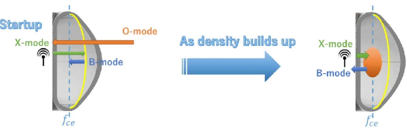
Fig. 1 Different fuel types consumed for certain geographic areas as reported by BP global 2016 ... 1 Fig. 2 Annual production of various types of energies over time, as reported by BP Global ... 2 Fig. 3 Cross section as a function in energy for fusion reactions of different H isotopes ... 4 Fig. 4 QUEST's cross sectional view showing different poloidal field coils and other in-vessel components ... 7 Fig. 5 Low field side phased array launcher of Klystron (8.2 GHz) [36] ... 7 Fig. 6 O-mode injection from low field side, with purple as low density plasma and orange as high density plasma. It can be seen that at low density, resonance layer (𝑓𝑐𝑒) is attainable, but at high density, reflection occurs ... 9 Fig. 7 Dispersion relation for the ordinary O mode propagating perpendicular to magnetic field (from ref. [30], where vg is group velocity and vph is phase velocity) ... 10 Fig. 8 Dispersion relation for the extraordinary X mode propagating perpendicular to the magnetic field (from ref. [30], where 𝛺𝑐𝑒 is the ion cyclotron frequency) ... 11 Fig. 9 X-mode launch from low field side such that increasing the wave frequency to the 2nd harmonic would provide access to the second harmonic resonance layer. ... 11 Fig. 10 The orientation of the electrostatic electron Bernstein wave (EBW) ... 13 Fig. 11 The formation of LHW 𝜔1 and two sidebands 𝜔2 and 𝜔3 at the EBW mode conversion point such that 𝜔0 is the pump wave (from ref. [57]). ... 14 Fig. 12 The PDI spectrum showing the LHW wave at frequency 𝜔1, and sidebands at frequencies 𝜔2 and 𝜔3 where 𝜔0 is the pump wave. ... 14 Fig. 13 Time evolution of plasma building up density from O-X-B conversion from LFS where the figure to the left shows the ray path during under-dense plasma for a reflective mirror polarizer at the HFS, and as the density builds up, the ray path changes to be as the right figure represents.

... 17 Fig. 14 Poloidal projection of EBW ray-tracing results for the X-mode launched form HFS perpendicular to magnetic field (from ref. [69]). ... 18 Fig. 15 EBW assisted plasma current startup schematic. Poloidal projection of EBW ray-tracing based on the plasma equilibrium reconstructed from experimental data (from ref. [45]) using 28 GHz gyrotron and 100 kW RF power. ... 19 Fig. 16 Time evolution of plasma building up density from X-B conversion from HFS ... 19 Fig. 17 QUEST poloidal field profile is shown with dark red representing flux loop positions such that FLT is flux loops top, FLC is flux loops center, FLB is flux loops bottom, FLS is flux loops side, FLTS is flux loops top-side and FLBS is flux loops bottom-side. ... 20 Fig. 18 Different time snaps of a magnetic reconstruction output from EFIT to demonstrate the

(9)

vi

time evolution of the last closed flux surface (LCFS) where the blue line represents the last closed

flux surface and the red lines represent the layout of the QUEST vessel ... 22

Fig. 19 Flux loop peaks such as (left) center flux loops (FLC), (left-middle) top (FLT) and bottom (FLB) flux loop peaks, (middle-right) Top side bad bottom side flux loop peaks (FLTS and FLBS), and (right) is side flux loop peaks (FLS) such that red is the measured signals after integration and drift removal, and blue is the calculated mutual flux that matches this shot at the flux loop positions. The x-axis in those figures resembles the flux loop numbers, while the y-axis resembles the flux value. ... 22

Fig. 20 The iterative feedback process of the GENRAY's tracing calculation... 24

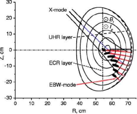
Fig. 21 (Right) Poloidal cross section of the HFS injected ray such that the dashed magenta line represents the fundamental ECR layer, the dashed blue line represents the UHR layer and the dashed red line represents the X-cutoff layer. (Left) Toroidal cross section ... 25

Fig. 22 Average current density as a function in major radius ρ for two injection angles at plasma density of ne=5×1017m-3 and plasma temperature of 50eV. The sign of Javg indicates the direction of propagation (+ve is clockwise and -ve is counter clockwise) ... 25

Fig. 23 Plasma current as a function in density, where ne is the peak value of the density’s assumed Gaussian profile. ... 26

Fig. 24 Poloidal view of ray not accessing UHR due to density build-up such that; mag. surf. is the magnetic surface calculated by GENRAY, LCFS is the last closed flux surface, 1st harm. and 2nd harm are the fundamental and 2nd ECR harmonic layers ... 26

Fig. 25 Setup for power delivery from LFS to HFS in QUEST showing the two klystrons labelled K1 and K2, a waveguide switch to switch between LFS and HFS, an arc detector connected to an interlock system for safety, a DC blocker, and the antennas with the ECRL position shown in perspective. ... 28

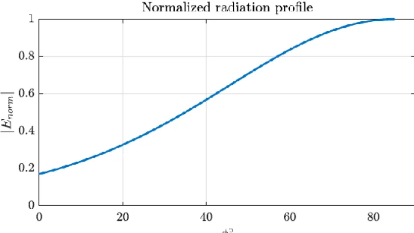
Fig. 26 Normalized open-ended waveguide radiation profile as a function in ϕ ... 30

Fig. 27 Normalized absorbed power as a function in ϕ ... 30

Fig. 28 ECR absorption as a function in electron temperature ... 31

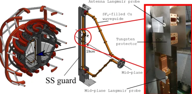
Fig. 29 HFS waveguide assembly in QUEST such that SS guard is the stainless steel guard, Port is where the flange connecting vacuum side and atmospheric side is, and Antennae are where the open-ended waveguide locations are (behind the SS guard). ... 32

Fig. 30 Design of the waveguide antenna with the tungsten plate protector installed and two Langmuir probes installed (one at the antenna’s vertical position and the other at the mid-plane’s vertical position) ... 32

Fig. 31 HFS waveguide design in QUEST showing the location of the RF leak monitor outside of the vessel. ... 33

Fig. 32 Leakage vs total input power for different vacuum shots with different input powers... 34 Fig. 33 Langmuir probe's characteristics of the current-potential curve, where the dotted red line

(10)

vii

represents the slope required for the calculation ... 35 Fig. 34 Langmuir probe design showing the alumina support, one out of four crimps and one out of four tungsten pins that have only 1.6mm exposed to plasma ... 35 Fig. 35 Final assembly of the Langmuir probe ... 36 Fig. 36 Connecting circuit for the Langmuir probe such that Vf is the floating voltage, Is the ion saturation current and Ch is the oscilloscope’s connecting channel ... 36 Fig. 37 Different spectrum analyzer connecting schemes such that A) has the spectrum analyzer connected to the LFS waveguide, which would allow for both LFS and HFS injections as non- used LFS waveguides are available, B) spectrum analuzer is connected to the HFS lower antenna, allowing for only half of the HFS injection power to be injected, and C) spectrum analyzer is connected to the HFS lower antenna with 100% of the LFS system operating. ... 37 Fig. 38 Full spectrum of PDI where 𝜔1 is the lower hybrid angular frequency, 𝜔2 is the sideband frequency and 𝜔0 is the central frequency (8.2 GHz in this work) (from ref. [57]) .. 38 Fig. 39 The grounded pins of the antenna probe were removed, and its connection to the oscilloscope was replaced with the 350 MHz oscilloscope to try and measure the lower hybrid wave (LHW) ... 38 Fig. 40 A typical waveform of the different plasma control parameters and diagnostics for a single shot for both LFS and HFS such that a) is the toroidal field, b) is the poloidal field (PF2-6), c) is the total klystron power, d) is the leakage from RF monitor, e) is the Hα sensor, f) is the oxygen sensor, g) is the plasma current, h) is the electron temperature, i) is the interferometer’s line- integrated electron density and j) is the Langmuir probe’s local electron density (at the antenna position Z=19cm) ... 39 Fig. 41 Camera image for toroidal field current of RECRL=0.55m for (a) LFS and (b) HFS at 33 kW of injected 8.2 GHz RF power. ... 40 Fig. 42 Comparison between interferometer (IF) density and plasma edge (camera) density calculation for HFS and LFS... 41 Fig. 43 Langmuir Probe's electron temperature for HFS and LFS where RECRL = 0.55m, Pt = 33 kW and no poloidal field ... 42 Fig. 44 Comparison between HFS and LFS in terms of time evolution of leakage power ... 42 Fig. 45 Power dependency of the leakage for HFS and LFS during plasma discharges where the dashed lines are the best fit lines for both HFS and LFS cases. ... 43 Fig. 46 The red arrows show the distance between the injection systems and the ECRL (dashed cyan line) ... 44 Fig. 47 Leakage for HFs and LFS by changing the toroidal field current, which would then change the position of the ECRL (RECRL) ... 44 Fig. 48 Poloidal field dependence at total klystron power and ECRL position of RECRL=0.55m.

(11)

viii

Both Hα and OII show BPF2-6 dependency, however, it is not so significant and while Ip show’s a significant dependence. It shall be noted that even though it is clear that smaller values of BPF2-6

result in higher Ip, we shall stop at 0.38mT as the results will be affected once the other steps are conducted. ... 45 Fig. 49 Toroidal field (TF) dependence at total klystron power and BPF2-6=0.38mT. Leak does not show any significant dependency on the toroidal field strength, while Hα and OII show a positive tendency towards higher toroidal field strength. However, Ip, the most important factor in this scan, shows an optimum position around RECRL=0.44m ... 46 Fig. 50 Poloidal field dependence at total klystron power and ECRL position of RECRL=0.44m. Ip, in this test as well, showed a tendency towards an optimum BPF2-6 that does not agree with Hα and OII, nonetheless, as mentioned previously, Ip is of highest priority. Leak does not show any dependency. ... 47 Fig. 51 Gas puff dependence at total klystron power, RECRL=0.44m and BPF2-6=0.78mT ... 47 Fig. 52 HCUL dependency of Ip for the HFS case ... 48 Fig. 53 Fast camera image comparison between a) LFS and b) HFS for RECRL=0.44m, BPF2- 6=0.78mT and GP=24ms ... 48 Fig. 54 Shot number 38934: 10ms HFS injection at BPF2-6=0.78 mT, RECRL=0.44 m, GP=24ms such that a) is leakage monitor measured in volts, b) H radiation sensor measured in volts, c) oxygen sensor measured in volts, d) Langmuir probe’s electron temperature measured in eV (at Z=19cm) and e) Langmuir probe’s electron density measured in m^-3 (at Z=19cm). The right y- axis in all those figures show plasma current measured in kA. ... 49 Fig. 55 Shot number 38939: 10ms LFS injection at BPF2-6=0.78mT, RECRL=0.44m, GP=24ms such that a) is leakage monitor measured in volts, b) H radiation sensor measured in volts, c) oxygen sensor measured in volts, d) Langmuir probe’s electron temperature measured in eV (at Z=19cm) and e) Langmuir probe’s electron density measured in m^-3 (at Z=19cm). The right y-axis in all those figures show plasma current measured in kA. ... 50 Fig. 56 Shot number 38795: 100ms HFS injection at BPF2-6=0.78mT, RECRL=0.44m, GP=24ms such that a) is leakage monitor measured in volts, b) H radiation sensor measured in volts, c) oxygen sensor measured in volts, d) Langmuir probe’s electron temperature measured in eV (at Z=19cm) and e) Langmuir probe’s electron density measured in m^-3 (at Z=19cm) . The right y- axis in all those figures show plasma current measured in kA. ... 52 Fig. 57 Shot number 38796: 100ms LFS injection at BPF2-6=0.78mT, RECRL=0.44m, GP=24ms such that a) is leakage monitor measured in volts, b) H radiation sensor measured in volts, c) oxygen sensor measured in volts, d) Langmuir probe’s electron temperature measured in eV (at Z=19cm) and e) Langmuir probe’s electron density measured in m^-3 (at Z=19cm) . The right y- axis in all those figures show plasma current measured in kA. ... 53

(12)

ix

Fig. 58 The snapshots of the fast camera of shot 38941 ... 54 Fig. 59 A scale was installed to measure the distance, while capturing the camera image from the exact same position as the plasma shots. This is to translate pixels to distance ... 55 Fig. 60 The time evolution of Rmax where Rmax is the radial position of the brightest point at the mid-plane ... 55 Fig. 61 LFS and HFS spectrum analyzer results such that ‘LFS’ indicates 3 klystrons injecting from LFS while connecting the spectrum analyzer from the HFS and ‘HFS’ indicates only one klystron firing from HFS because the spectrum analyzer is connected to the HFS, and another two are firing from LFS. ... 56 Fig. 62 LHW frequency vs R where Rmax is the same as that in Fig. 60 and BW1 is the LHW bandwidth ... 57 Fig. 63 (Upper) the Langmuir probe antenna's waveform as captured by the oscilloscope, and (Lower) is the spectrum after FFT conversion. The no plasma shot was included for reference.

The dotted-black line shows the expected LHW bandwidth only without any magnitude expectations. ... 58 Fig. 64 SA reading of HFS and LFS such that the dotted black line is the expected sideband bandwidths. ... 58 Fig. 65 (Top) Ideal low pass filter spectrum (right) and wavegorm (left) for a cutoff frequency of 50MHz, and (bottom) ideal high pass filter for the spectrum (left) and waveform (right) for a cutoff frequency of 50MHz. The bottom right figure has the no plasma at 0mV so it is invisible as it lies behind the HFS and LFS signals, and the right yaxis and the purple curve show the Hα time evolution of this shot. ... 59 Fig. 66 (Left) Ip for forward polarity of the poloidal field, peaking at 1.1 kA, and (Right) Ip for reverse polarity of the poloidal field peaking at -1.06 kA ... 60 Fig. 67 Fast camera snapshot results for HFS with PF4 (shot 38957) for nine instances from 0.333ms to 2.000ms ... 61 Fig. 68 Fast camera snapshot results for HFS with PF4 (shot 38973) for nine instances from 0.333ms to 2.000ms ... 62 Fig. 69 Shot number 38957: HFS injection at BPF2-6=1.5mT, BPF1-7=0.0863mT, RECRL=0.44m, GP=24ms, and BPF4=- 0.6578mT such that a) is leakage monitor measured in volts, b) H

radiation sensor measured in volts, c) oxygen sensor measured in volts, d) Langmuir probe’s electron temperature measured in eV (at Z=19cm) and e) Langmuir probe’s electron density measured in m^-3 (at Z=19cm) . The right y-axis in all those figures show plasma current measured in kA. ... 63 Fig. 70 Shot number 38959: HFS injection at BPF2-6=1.5mT, BPF1-7=0.0863mT, RECRL=0.44m, GP=24ms, and BPF4=- 0.6578mT but starts rising 10ms earlier than 38957. a) is leakage monitor

(13)

x

measured in volts, b) H radiation sensor measured in volts, c) oxygen sensor measured in volts, d) Langmuir probe’s electron temperature measured in eV (at Z=19cm) and e) Langmuir probe’s electron density measured in m^-3 (at Z=19cm) . The right y-axis in all those figures show plasma

current measured in kA. ... 64

Fig. 71 Shot number 38973: LFS injection at BPF2-6=1.5mT, BPF1-7=0.0863mT, RECRL=0.44m, GP=24ms, and BPF4=- 0.6578mT and starts at the same timing as shot 38959. a) is leakage monitor measured in volts, b) H radiation sensor measured in volts, c) oxygen sensor measured in volts, d) Langmuir probe’s electron temperature measured in eV (at Z=19cm) and e) Langmuir probe’s electron density measured in m^-3 (at Z=19cm) . The right y-axis in all those figures show plasma current measured in kA. ... 65

Fig. 72 Time evolution of the center stack loop voltage. It started from 2.99s while the RF power injection started at 3.0s. This loop voltage is the equivalent of a magnetic field of 1.495mT at the mid-plane and the ECRL position. ... 66

Fig. 73 A 3D image of the plasma video for HFS injection (shot 38941) after only considering the mid-plane slice, where x-axis is time, y-axis is pixels representing the radial axis, and z-axis is brightness. ... 67

Fig. 74 Comparison between LFS (shot 38939) and HFS (shot 38941) for the mid-plane slice of the camera video such that the x-axis represents time, y-axis represent radius R, and the color axis represents camera image brightness ... 67

Fig. 75 The brightness for LFS (shot 38939) vs HFS (shot 38941) as a function in the radius R at time t=1.503s ... 68

Fig. 76 Interferometer data analysis for LFS (shot 38939) vs HFS (shot 38941) where (top) is line-integrated density, (middle) the path length of the interferometer signal inside the plasma [one-way], and (bottom) is the line-averaged density at a threshold of 20% ... 69

Fig. 77 Peak density as a function in the threshold percentage ... 70

Fig. 78 The position of the HFS-installed Langmuir probe compared to the UHRL ... 70

Fig. 79 Time evolution of OII and Ip for the 100ms shot ... 71

Fig. 80 The maximum brightness radial position for different poloidal fields ... 72

Fig. 81 Time evolution of the interferometer's line integrated phase difference compared to the RF monitor's ... 72

Fig. 82 The convolution between the RF leakage monitor and the phase difference of the interferometer, showing that they both are in synchrony as the maximum value of the convolution is at time 0.5ms ... 73

Fig. 83 Pixels vs time for HFS shot 38795. Note that pixels indicate the vertical displacement (Z- axis), however, an accurate translation from pixels to Z is not available... 74 Fig. 84 Pixels vs time for LFS shot 38796. Note that pixels indicate the vertical displacement (Z-

(14)

xi

axis), however, an accurate translation from pixels to Z is not available... 74 Fig. 85 Same as Fig. 84 but the brightness is amplified ... 75 Fig. 86 (Top) waveforms of interferometer phase shift, Leak and Rmax after normalizing the amplitude and removing the bias, and (bottom) is the FFT to check whether the signals are in synchrony ... 75 Fig. 87 (Left) Spatial distribution of flux and (right) nindex at BPF2-6=0.78mT and BPF1-7=-0.43mT ... 77 Fig. 88 Modified HFS injection system showing a tilted antenna from the bottom to free up the CS space for better magnetic reconstruction ... 78 Fig. 89 For propagation along the magnetic field, Left Circularly Polarized (LCP) wave rotates in the counterclockwise direction, while the Right Circularly Polarized (RCP) wave rotates in the clockwise direction, for an observer looking at the outgoing wave. 𝐵0 is the magnetostatic field.

𝐸𝑡 is defined as the transverse electric field. This figure is (from ref. [30]) ... 92 Fig. 90 Schematic for ECRL penetration bench test ... 95 Fig. 91 The water load used to terminate the waveguide while showing the positions of the temperature sensors T1 and T2 ... 95 Fig. 92 The final design of the water load, waveguide and the electromagnet ... 96 Fig. 93 Temperature difference as a function in time for pulse durations of T=10s, T=30s, and T=60s for a water load terminating a waveguide with input RF power of 20kW that is subject to a magnetic field of 0.3T ... 96 Fig. 94 Energy as a function in pulse duration (blue) with dotted-black line as best fit line for measuring slope and detecting the power ... 97

(15)

(16)

1

1. Introduction

Cumulative greenhouse gas emissions are a direct contributor to the global rise in temperature [1]–[3]. The united nations agreed that there is an average rise of 2ºC in the global temperature [4]. A significant reduction in fossil fuel consumption is required to regulate the temperature rise.

Less than half of the gas reserves, less than two thirds of oil reserves and only 20 percent of coal reserves is to be consumed to avoid surpassing the 2ºC rise in temperature, and this rate should be maintained until 2050 [5]. The aggressive consumption of fossil fuels is a strong indicator of the huge energy demand, as reported by U.S Energy Information Administration (EIA), which presents a difficulty to meet the conditions required for suppressing the average temperature rise.

Fossil fuel consumption constitutes more than 50% of the global energy market, as reported by BP global in 2016 (see Fig. 1 ).

Fig. 1 Different fuel types consumed for certain geographic areas as reported by BP global 2016 Solar, wind, tidal, geothermal, and thermonuclear fusion constitute a clean and environmentally friendly renewable sources of energy that can be used as an alternative to fossil fuels.

Combustibles, renewables, hydro and nuclear energy plants show their annual market in Fig. 2 as reported by BP global [6].

More than a century ago, nuclear physicists understood that nuclear reactions can be controlled to generate a significant amount of energy. To put things into perspective, annually, about 109,136 TWh of energy are estimated to be consumed worldwide (as of 2015), while the sun, fueled by nuclear reactions, generates about 1.06×10¹¹ TWh per second, which is more than the entire energy consumption in the history of the planet. Aside from the capability of putting this much energy into military applications, resulting in hundreds of thousands of deaths from the Hiroshima and Nagasaki fission bombs, which progressed even further by the construction of Hydrogen fusion bombs that are potentially a thousand fold more powerful, the peaceful application of

(17)

2

harnessing this energy for improving the lifestyle of civilians is also in tremendous progress.

Nuclear fission energy was controlled for the production of commercial energy in the mid-19^th century. The progress within harnessing fission energy led to the idea that fission energy would be safe and available within the advancement of technology, however, that has not been the case

as the fission production not only stagnated in developing its technology, but also languished in the past decade from 18% to about 14% in terms of total world energy consumption [6]. On the other hand, thermonuclear fusion energy yield has been widely known to be unparalleled since the 1950s [1], not to mention its virtually nonexistent carbon footprint [2].

Moreover, fusion technology gained a lot of credibility after revealing how operationally safe it is in terms of explosions and dealing with radioactive materials [3]. However, fusion energy has been researched for more than 60 years and still has several milestones to surpass before realizing commercialization, yet it is still thought of as a promising source of energy that is to be deployed [4], [7]. Aside from fusion skeptics claiming that integrating fusion energy in the grid is an absolute impossibility, the fact of the matter is that there are plenty of unsolved problems that are being tackled one at a time, but that is a strong indicator that there is no profound knowledge about how to properly build a reactor. However, it can be said with a high degree of confidence that fusion, if realized, will be expensive in comparison to its competitors. For that reason, plenty of innovative research is conducted with the motive to reduce the reactor cost by making the reactor design more compact, by changing the materials used to constructing it, or by changing the plasma heating methods. A detailed review about different reactor designs is to be presented

Fig. 2 Annual production of various types of energies over time, as reported by BP Global

(18)

3

in section 1.2. Furthermore, different plasma heating technologies are to be explored in attempt to improve the results of the economic reactors. This work will focus on economically heating and driving plasma current in the case of compact reactors.

1.1 Fusion Theory

This section will discuss the basic theory of nuclear fusion and how the fusion equations can be put to use to create a nuclear reactor and generate power.

1.1.1 Thermonuclear fusion reaction

Thermonuclear fusion reaction, based on Einstein’s famous E=mc¬2 equation, goes as follows:

𝐷₂

1 + 𝑇¹ ₃²𝐻𝑒₄ (3.5 𝑀𝑒𝑉) + 𝑛⁰ ₁ (14.1 𝑀𝑒𝑉) 1.1.1

𝐷₂+ 𝐷₂𝐻𝑒₃+ 𝑛₁+ 3.27 𝑀𝑒𝑉 1.1.2

𝐷₂+ 𝐻𝑒₃𝐻𝑒 + 𝐻₁+ 18.3𝑀𝑒𝑉 1.1.3

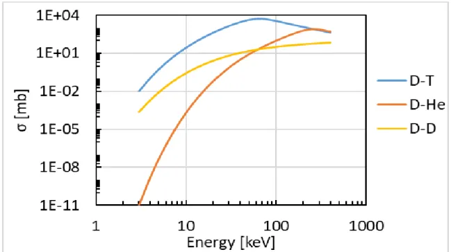
where D (deuterium) and T (tritium) are Hydrogen isotopes, n is neutron. The primary difficulty with achieving this reaction is that to overcome the coulomb forces repelling the nuclei, a temperature in the order of 10⁶°C is required which can be considered as an external catalyzing factor to the reaction. It can be seen that several versions exist based on the Hydrogen isotope input, making D-He the most attractive as it has the largest energy yield. However, considering the cross-section between nuclei as a function in energy is essential since the catalyzing factor is difficult to achieve. The cross-section is defined as

𝜎 =𝑆(𝐸)

𝐸 ∗ exp (−𝐵𝐺

√𝐸) 1.1.4

where 𝜎 is the cross-section, S is the astrophysical S-function, and BG is the Gamov constant.

The Gamov constant is defined as

𝐵𝐺 = 𝜋𝛼𝑍₁𝑍₂√2𝑚𝑟𝑐² 1.1.5

where Z1 and Z2 are the atomic numbers of the two nuclei to be fused. The cross-section calculations, based on [7] are as shown in Fig. 3.Based on Fig. 3, despite D-He dominating in terms of energy yield, it can be seen that D-T has higher sigma as energy decreases, making its fusion condition achievable at comparatively lower temperature. Correspondingly, D-T fusion is to be the focus of this work, where the bioavailability and cost of both is to be considered.

(19)

4

1.1.2 Thermonuclear fusion ignition

Thermonuclear fusion is particularly attractive in the field of renewable energies because once a certain condition is achieved (ignition), the plasma will reach a state where it can internally self- sustain its temperature against the energy losses. Ignition would in turn allow for the removal of the applied heating, significantly reducing the input power. This sustained condition is due to the emission of the He4 particle (alpha particle [8]) in the D-T reaction such that

𝑃_𝐻+ 𝑃_𝛼 = 𝑃_𝐿 1.1.6

where 𝑃𝐻 is the heating power, 𝑃𝛼 is the power generated by the alpha particle, and 𝑃𝐿 is the power loss. Achieving ignition condition depends on several factors including the size and structure of the reactor, plasma temperature, plasma density and the magnetic field strength.

However, a reliable indicator of how well a particular reactor is performing is the Lawson criterion (also known as the triple product)

𝑛𝑇𝜏 ≥ 3 × 10²¹𝑘𝑒𝑉 𝑠

𝑚³ 1.1.7

where T is ion temperature in eV, 𝜏 is plasma confinement time, and n is ion density [9]. This critical criterion not only indicates the threshold for self-sustained fusion, but also indicates the possibility to trade off different parameters. This is particularly useful as each reactor has its unique structure and specifications mastering one or two of the triple-product parameters.

Noteworthy is to say that not a single reactor was yet able to produce plasma with satisfying values to all three key parameters simultaneously.

Fig. 3 Cross section as a function in energy for fusion reactions of different H isotopes

(20)

5

1.2 Thermonuclear fusion reactors

Given that no solid material can endure the extreme particle and heat loads produced by high temperature and density of fusion plasmas, plasma confinement is a necessity. Fusion devices are majorly divided into Magnetic Confinement Fusion (MCF) plants and Inertial Confinement Fusion (ICF) plants. Examples of ICF devices are such as (laser-driven [10] or Z-pinch [11]).

However, MCF devices have proven to have a higher Lawson criterion than ICF ones [12], [13]

and therefore MCFs are the focus of this work. Furthermore, toroidal machines are to be focused on rather than open-field machines [14]. Not to mention, toroidal machines vary in shape and structure giving several standard reactor types like tokamaks [15], stellarators [16], [17], reversed field pinch [18], spheromaks [19] and others [20].

1.2.1 Tokamaks

Tokamak is a Russian term which translates to ‘toroidal magnetic container’. Credit goes to Soviet physicists I. Y. Tamm and A. Sakharov (who were inspired by an original idea of O. Lavrentyev [21]) to create the Tokamak concept. Historically, ever since the T-3 tokamak belonging to Kurchatov Institute – Russia obtained a plasma temperature of 1 keV [22], tokamak research was the focus of many nuclear fusion research institutes [23]–[26]. Tokamaks-based D-T reactions were able to supply an output power of the order of MW [15], [27]. Furthermore, ITER, the world’s largest nuclear fusion reactor that is to be the first to achieve output power 10 fold that of the input power, is in fact a tokamak [28].

Essentially, tokamaks contain the superposition of both toroidal and poloidal fields (TF and PF respectively). The toroidal flow of plasma (plasma current) creates a PF which contributes to the net PF profile. Applying TFs solely is incapable of confining plasmas as it has a gradient (the center of the tokamak being of strongest magnetic field B), which would cause ions and electrons to drift vertically in opposite directions due to the ∇𝐵 drift. This charge separation would create a vertical electric field, which would then interact with B causing the plasma to drift radially outwards towards the tokamak walls (this is known as the 𝐸 × 𝐵 drift. To counter this phenomenon, driving plasma current toroidally would a plasma PF that would nullify the effect of the 𝐸 × 𝐵 drift, and would in turn create spiraling magnetic lines. In addition, plasma in this situation would drift outwards with hoop force, which is why the installation of toroidal coils to create PFs is necessary. Conventionally, tokamaks have a solenoid located at its center, which is responsible to drive plasma current, referred to as the center solenoid (CS) or center stack.

Another function that the CS serves is the initiation of plasma breakdown, which is referred to as inductive (Ohmic) breakdown. However, a limitation of primarily depending on CS for heating and plasma current drive is that its coil current cannot be changed indefinitely. Another limitation for Ohmic heating and current drive (Goldston, 1984) is that plasma particle friction decreases as the temperature increases. This limitation dictates the use of other heating methods, referred to as non-inductive heating methods (van Houtte, et al., 2004). The primary non-inductive heating methods in the market are: (a) Neutral Beam Injection (NBI), which is used to inject neutral particles that are immune to the magnetic field restrictions and hence can roam freely inside the plasma, colliding with the charged particles and then heating up plasma, and (b) Radio frequency

(21)

6

(RF) wave injection, which injects RF waves of high power that are to be absorbed by the plasma at certain resonance conditions, which would heat up the plasma.

1.2.2 Spherical tokamaks

The primary issues with conventional tokamaks is that they are unstable in high  as well as expensive, hence the introduction of spherical tokamaks. Spherical tokamaks (STs) are defined as tokamaks with low aspect ratio. Aspect ratio in this context is 𝐴 = 𝑅₀/𝑎, where 𝑅₀ and 𝑎 are the major and minor radii of the tokamak respectively. A tokamak is considered spherical when 𝐴 < 1.5, such that its cross-sectional view is D-shaped. STs are stable as they are of high β [29]. β is defined as the ratio between plasma pressure and magnetic pressure. Another fundamental advantage of STs is that high-β plasmas share similar characteristics to low-β plasmas but at significantly lower magnetic fields, hence reducing the overall cost of the reactor.

In addition, the low aspect ratio gives little room for a CS, which would create Ohmic heating and current drive issues [30]. This pushes the incentive to heat high-β plasmas using purely non- inductive methods. Not to mention, if ST operation could be conducted CS-free, that would further improve its economic value. A list of all the famous tokamaks are listed and compared in [31].

1.2.4 QUEST spherical tokamak

QUEST (Q-shu University Experiment with Steady State Spherical Tokamak) is a medium-sized ST with a purpose of studying steady-state operation issues, plasma-wall interaction phenomena in steady state which is of critical importance for realizing a volume neutron source full scale fusion plant [32]–[34]. Another theme for QUEST is non-inductive heating and current drive [29], [35].

The device parameters are: major radius 𝑅₀= 0.68𝑚, minor radius 𝑎 = 0.40𝑚 and toroidal magnetic field of 𝐵_𝑇 = 0.25𝑇 in steady state (and 0.5𝑇 for up to 1s at a radius of 𝑅 = 0.64𝑚).

The radius of the outer surface of the CS and the radius of the inner surface of the wall are 0.22m and 1.4m respectively. Flat diverter plates that are tungsten-coated for high heat load endurance) are located at a vertical displacement of 𝑍 = 1𝑚 (where the mid-plane is located at 𝑍 = 0m).

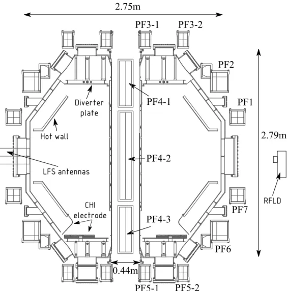
QUEST has a total of 16 toroidal coils such that the spacing between pairs is 45°. QUEST has 11 PF coils and a pair as shown in Fig. 4. QUEST is equipped with RF sources of 2.45 GHz klystron of 50 kW, 8.2 GHz klystron of 55 kW and 28 GHz gyrotron of 250 kW.

For controlled 8.2 GHz launching in QUEST, a launching antenna is used (see Fig. 5). For launching polarization control, mixing two orthogonal electric field components with different phase is crucial. This orthogonal electric field mixing is done through a device called orthomode transducer. The previous Kyushu University tokamak (called TRIAM-1M) adopted its Lower Hybrid Current Drive (LHCD) system to QUEST. This system is to be used for Electron Bernstein Wave Heating / Current Drive (EBWH/CD) in QUEST at an operating frequency of 8.2 GHz (details are to be discussed in a later section). A number of rectangular waveguides (16 in total), called WR-137, were used for the power transmission of 200 𝑘𝑊 to the LHCD system. The attenuators and phase shifters found in the transmission line were used to control the output polarization state at the orthomode transducer. The orthomode transducer conceptual design part was illustrated in Fig. 5, where two field components with different intensity and phase at the rectangular waveguide input were mixed at the orthomode transducer, and were driven to the antenna given an arbitrary elliptical polarization state.

(22)

7

Fig. 4 QUEST's cross sectional view showing different poloidal field coils and other in-vessel components

Fig. 5 Low field side phased array launcher of Klystron (8.2 GHz) [36]

(23)

8

1.3 Motivation

Several complications can arise from inductive heating [37] since in STs, Ohmic heating is suitable only for startup because as temperature increases, resistance decreases, and the Ohmic heating becomes less effective, which is why ohmic heating can be available to control plasma current and its profile, rather than plasma start-up. As a consequence, there were over 100 non- sustained breakdown shots on JET experiments in 2009 [37], which is why non-inductive heating is prevailing. One non-inductive heating method is known as Neutral Beam Injection (NBI), which was proven effective in terms of global energy confinement scaling [38] as well as local transport scaling [39] since the 80s. A primary drawback for NBI which was known since 1987, however, is that if the plasma density was not above a certain threshold (𝑛_𝑒~10¹⁹𝑚⁻³), NBI heating will be rendered ineffective [40]. Another non-inductive heating method is the injection of radio frequency RF electromagnetic waves (EMW) into the plasma, where if certain conditions were met, resonance between EMWs and plasma particles occur (LHW can interact with electrons via Landau damping), driving the plasma particles to collide with each other and therefore elevate the plasma temperature as a result (where the electron can directly absorb the RF heat). This method of heating is primarily divided into: Landau damping [41], transit-time magnetic pumping, ECRH heating (Electron Cyclotron Resonance Heating) [42], and ICRH (Ion Cyclotron Resonance Heating) [43] and IIHH (Ion-Ion Hybrid Resonances) [44], where ECRH is the most famous among all three techniques, given that electron mass is much smaller than ion mass, and therefore building the resonance layer is easier. The primary advantage of RF heating is that it requires no minimum density threshold to operate, which seems to be an attractive feature compared to NBI heating. On the other hand, RF heating has an upper density limit where if surpassed, a reflection layer will be created, preventing EMWs to reach the plasma resonance layer, and therefore rendering the whole technique ineffective. Since both heating techniques (NBI and RF) have opposite problems, where one suffers from low density (NBI), and the other suffers from high density (RF), it comes as no surprise to have a hybrid heating system consisting of both RF and NBI. The scheme is as follows: Plasma in a ST is to be heated using ECRH for density to develop until reaching a certain threshold where the reflection layer prevents ECRH from continuing, during which, a shift to NBI is to be done. Another issue that arises from that hybrid is that the upper density limit for ECRH is sometimes lower than the lower density limit for NBI, depending on the operating frequency of the RF source. In order to tackle this issue, different modes of operation for the EMWs of ECRH are to be thoroughly discussed where the upper density limit can be manipulated and in some optimal cases completely removed. The focus of this work will be to manipulate the different modes of EMWs targeting higher plasma density during the ECRH phase in attempt to overcome the plasma density cutoff limit. Moreover, the concept of Electron Bernstein Wave is to be discussed in details as it plays a key role in achieving higher plasma densities during the RF wave injection phase. Highly efficient excitation of electron Bernstein wave is the primary goal with heating and current drive as the targets.

(24)

9

2. Plasma’s RF modes of propagation

There are various modes of propagation of RF waves inside a plasma depending on the polarization, injection position with respect to the magnetic field, injection angle, etc. Some of those modes are to be discussed in detail in this section as the mode selection process significantly depends on the properties of those modes.

2.1 Conventional O-mode heating and current drive

Ordinary O-mode, basically known as electron cyclotron resonance heating (ECRH), operates by polarizing the wave in a transverse electric magnetic (TEM) form such that the wave electric field is linearly polarized along B0.

Fig. 6 O-mode injection from low field side, with purple as low density plasma and orange as high density plasma. It can be seen that at low density, resonance layer (𝑓_𝑐𝑒) is attainable, but at high density, reflection occurs

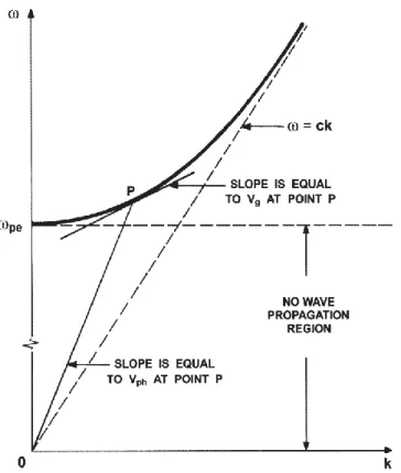
The dispersion relation of O-mode, as shown in Fig. 7, is simply expressed as

𝜔²= 𝜔_𝑝𝑒²+ 𝑐²𝑘² 8

(25)

10

Fig. 7 Dispersion relation for the ordinary O mode propagating perpendicular to magnetic field (from ref. [30], where vg is group velocity and vph is phase velocity)

In general, O-mode is simple and effective, but a major drawback is that as density starts to build up, plasma acts as a reflector and RF wave loses access to ECR layer. Therefore, a different mode is required if the target is high density.

This non-inductive plasma heating method have been actively performed in different tokamaks such as MAST [45], TST-2 [46], LATE [47], and QUEST [48], [49]. In [50], a plasma current of 8 kA was reported using 8.2 GHz klystron with power of 70 kW in QUEST.

2.2 Conventional way -X-mode heating and CD

X-mode operates by polarizing the wave in a way such that electric field 𝐸_𝑡 has a longitudinal component (along 𝑘 ) and a transverse component (perpendicular to 𝑘 ), making this wave partially longitudinal and partially transverse. This is widely known as elliptical polarization. The dispersion relation of X-mode, as shown in Fig. 8, is simply expressed as

𝑐²𝒌²

𝜔² = 1 −𝜔_𝑝𝑒² 𝜔²

𝜔²− 𝜔_𝑝𝑒²

𝜔²− 𝜔_𝑈𝐻² 2.2.1

where 𝜔_𝑈𝐻²≡ 𝜔_𝑐𝑒²− 𝜔_𝑝𝑒² such that 𝜔_𝑐𝑒 is the electron cyclotron frequency.

(26)

11

Fig. 8 Dispersion relation for the extraordinary X mode propagating perpendicular to the magnetic field (from ref. [30], where 𝛺𝑐𝑒 is the ion cyclotron frequency)

X-mode has a special feature of accessing a layer called the Upper Hybrid Resonance Layer (UHRL), where 𝒌 → ∞.

For X-modes, increasing the frequency of the source gives access to higher harmonics and thereby nullifying the effect of reflection at high densities. Graphically, this is done by pushing the inaccessible part of the plasma to the left, while creating another resonance layer at a higher harmonic (see Fig. 9).

Fig. 9 X-mode launch from low field side such that increasing the wave frequency to the 2nd harmonic would provide access to the second harmonic resonance layer.

(27)

12

In X-mode, increasing the frequency seems like an appealing solution whereas resonance layer is accessible, and this process can be repeated at the 3^rd harmonic layer and so on for improved results. However, the drawback of this process is that increasing the source frequency reduces the absorption efficiency, which thereby reduces plasma heat and density. Another problem that arises from the same approach of increasing the frequency is that it is technically difficult to engineer a device with high frequency and high power at the same time therefore a different approach is still required.

Given that those two modes are not the only solutions of the dispersion relation, there is a third mode, however, that is conveniently separated from both modes because of polarization orientation difference.

In general, both X-mode and O-mode have the same issue of the inaccessibility of reaching the cyclotron resonance layer once the plasma density is developed due to the cutoff layer, however, X-mode has an attractive feature of conditionally reaching the UHRL, where resonance would occur, and an electrostatic wave called the Bernstein wave will be developed that propagates along the magnetic axis. This electrostatic wave has the merit of being a longitudinal wave and therefore has the immunity of not suffering any cutoff layers, which is why this mode is the target of this work.

2.3 Merit for using Electron Bernstein Wave

Electron Bernstein Wave (or EBW) was first studied by Ira B. Bernstein theoretically in 1958 [51]

and experimentally in 1964 [52]. EBWs are electrostatic waves in a magnetized hot plasma. To derive the EBW dispersion relation, it is necessary to understand the profile of the hot plasma dielectric tensor, expressed from [53] as

𝜖 = 𝑰 +𝜔_𝑝𝑒² 𝜔² 𝜁₀ ∑

[

𝑛²

𝜇 𝐼̃ 𝑍_𝑛 _𝑛 𝑖𝑛𝐼̃ 𝑍^′_𝑛 _𝑛 −𝑛√2

𝜇𝐼̃ (1 + 𝜁_𝑛 _𝑛𝑍_𝑛)

−𝑖𝑛𝐼̃ 𝑍^′_𝑛 _𝑛 (𝑛²

𝜇 𝐼̃ − 2𝜇𝐼_𝑛 ̃ ) 𝑍^′_𝑛 _𝑛 𝑖√2𝜇𝐼̃ (1 + 𝜁^′_𝑛 _𝑛𝑍_𝑛)

−𝑛√2

𝜇𝐼̃ (1 + 𝜁_𝑛 _𝑛𝑍_𝑛) −𝑖√2𝜇𝐼̃ (1 + 𝜁^′𝑛 _𝑛𝑍_𝑛) 2𝜁_𝑛𝐼̃ (1 + 𝜁_𝑛 _𝑛𝑍_𝑛) ]

∞

𝑛=−∞

2.3.1

where

𝜁𝑛= (𝜔 + 𝑛𝜔𝑐𝑒) (|𝑘⁄ _{| |}|𝑣𝑇2) 2.3.2

is the frequency distance from the 𝑛^th cyclotron harmonic resonance,

𝜇 = 𝑘_⊥²𝑣_𝑇²⁄2𝜔_𝑐𝑒 2.3.3

, plasma dispersion function is

(28)

13 𝑍_𝑛 = 𝑍(𝜁_𝑛) = 1

√𝜋 ∫ 𝑒^−𝑠² 𝑠 − 𝜁_𝑛𝑑𝑠

∞

−∞

2.3.4

, 𝐼𝑚(𝜁_𝑛) > 0 and 𝐼̃ = 𝑒_𝑛 ^−𝜇𝐼_𝑛(𝜇) and 𝐼_𝑛 is the 𝑛^th order modified Bessel function.

The hot dielectric tensor 𝜖 is not only function in 𝜔𝑐𝑒 and 𝜔𝑝𝑒, but also in the wave vector 𝒌 and the temperature 𝑣_𝑇, which leads to the electrostatic modes, a different dispersion relation solution. The rise of the Bessel term in 𝜖 presents a lot of different roots, the Bernstein waves (or B-modes), for a given harmonic, as well as a different root (the X-mode). Given short wavelengths (large gyro radii), the X-mode and the B-mode decouple, hence the mode conversion to B-mode, where the dispersion relation is expressed as

𝜇 =𝜔_𝑝²

𝜔² ∑ 𝑙²𝐼̃(𝜇)_𝑙 1 + 𝑙 (𝜔_𝑐

𝜔)

∞

𝑙=−∞

2.3.5

where the approximations are: the electrostatic approximation where 𝑬 || 𝒏 and 𝑍_𝑛 ≅ −1/

ξ

_𝑛. EBWs are waves generated from the coherent motion of electrons around their guiding centers, which makes them longitudinal waves. The electrons gyrate around perpendicular magnetic field lines such that the Larmor radii are 𝜌 =^𝑐𝑚^𝑒^𝑣^𝑇

𝑒𝐵 where it is assumed that all the electrons gyrate with the same Larmor radius for simplicity. Periodic charge accumulation is in the same direction as the wave vector 𝒌.

Fig. 10 The orientation of the electrostatic electron Bernstein wave (EBW)

A unique feature of EBW is that EBW wavelength is 4 × that of the electron Larmor radius, which would practically eliminate 𝐸 × 𝐵 drift given that 𝜔 > 𝜔_𝑐 [54]. To understand the concept of EBW, a comparison between non-magnetized plasma and magnetized plasma during electric field presence is useful. Non-magnetized plasmas obey Langmuir dispersion

𝜔²= 𝜔_𝑝²+ 3𝒌²𝑣_𝑇² 2.3.6

However, magnetizing the plasmas would convert electron orbits from back-forth motion to elliptical. These interactions between static magnetic fields and electric fields, distorting the electron orbit, is known as upper hybrid resonance (UHR) such that

(29)

14

𝜔 = 𝜔_𝑈𝐻𝑅= √𝜔_𝑝²+ 𝜔_𝑐² 2.3.7

Increasing the magnetic field causes Lorentz force to overpower the electrostatic force, thus turning the electron orbit to a fully circular form. In such case, EBW can propagate even in over- dense plasmas (𝜔 < 𝜔_𝑝) as long as (𝜔 ≤ 𝜔_𝑐), which is a key feature for improving plasma density.

The reason why such condition exists is because at 𝜔_𝑐 < 𝜔_𝑝, the electrons’ orbits are of radius larger than that of the Debye length, exporting the charge disturbance from the inside of the Debye sphere to the external space-charge.

2.3.1 EBW’s parametric decay instabilities

The process of exciting EBW produces stimulated electromagnetic emission (SEE) caused by the parametric decay process as the Bernstein waves become parametric instability pumps upon reaching a large enough amplitude [55]. Stubbe and Kopka suggested that EBW’s nonlinear scattering of the lower hybrid waves (LHW) might lead to their observed broad symmetric structure [56]. As electrons have significantly lighter masses as compared to the seemingly motionless ions, if electrons oscillate at 𝜔₀ and ions fluctuate at low frequency 𝜔₁, these may beat with oscillating electrons to form 𝜔₀± 𝜔₁ and 𝜔₀ = 𝜔₁+ 𝜔₂, which is the usual resonant mode-mode coupling process as shown in Fig. 11. The spectrum is then shown in Fig. 12

Fig. 11 The formation of LHW 𝜔₁ and two sidebands 𝜔₂ and 𝜔₃ at the EBW mode conversion point such that 𝜔₀ is the pump wave (from ref. [57]).

Fig. 12 The PDI spectrum showing the LHW wave at frequency 𝜔₁, and sidebands at frequencies 𝜔₂ and 𝜔₃ where 𝜔₀ is the pump wave.

For confirming EBW mode conversion, EBW’s parametric decay instability (PDI) is to be measured. That is, when the injected X-mode wave reaches the UHR layer, scattering occurs during EBW conversion, which causes a sideband to rise next to the central RF frequency [57]–

[63] (8.2 GHz in this work), which is to be measured.

(30)

15

2.4 Mode Conversion for EBW

Given that EBWs, by nature, are space charge waves, this means that they require magnetized plasma for propagation, making their excitation only possible inside of the plasma and not from an external source. Electrostatic radiating antennae exist but their inclusion inside of the vessel is obligatory, which is undesirable since millimeter waves are required for high temperature plasma, making the antenna size less than 0.1 mm (same order as that of the electron gyro radius). High temperature plasma, however, has the potential to destroy such antennae, which makes mode conversion into EBW from a different mode, excited externally, the only option for EBW excitation in fusion plasmas. In this section, mode conversion is to be analyzed.

2.4.1 O-X-B mode conversion

For EBW to be excited, a slow X-wave propagating towards the UHR layer is required, which, for the 1^st harmonic EBWs, is limited to low densities since for higher harmonics, the UHR will be completely enclosed by the R-cutoff for X-waves. A two mode conversion scheme was first proposed by Preinhaelter [64] where an O-wave is launched from outside of the vessel, with an oblique angle of incidence or a non-vanishing parallel refractive index 𝑛_||. The parallel refractive index 𝑛_|| determines the wave behavior, however, for simplicity, consider the perpendicular refractive index 𝑛_⊥ component along the wave propagation inside of the plasma. It was already established that at 𝑛_⊥= 0, 𝑋 = 𝜔_𝑝𝑒²/𝜔² and 𝑌 = 𝜔_𝑐𝑒/𝜔, L-mode cutoff corresponds to

𝑋 = (1 − 𝑛| |2)(1 − 𝑌) 2.4.1

, R-mode cutoff corresponds to

𝑋 = (1 − 𝑛_{| |}²)(1 + 𝑌) 2.4.2

and O-mode cutoff corresponds to

𝑃 = 0 2.4.3

which, according to the above equations, O-mode cutoff is independent on 𝑛||. Given that the cutoff position is the limit beyond which the wave cannot propagate, X-waves are to be reflected back from first L-mode cutoff whereas the O-mode will be reflected back from 𝑋 = 1. However, to make use of EBW’s feature of propagating in over-dense plasmas, O-modes are to be converted to X-modes at the O-mode cutoff position, which means that R-cutoff has to coincide with O- mode cutoff. The modified equation promoting O-X conversion would then be

𝑋 = (1 − 𝑛_{| |}²)(1 + 𝑌) = 1 2.4.4

which would in turn make the optimum parallel refractive index