Learning about Conic Sections with Geometric Algebra and Cinderella (Innovative Teaching of Mathematics with Geometric Algebra)

se

Learning

about

Conic

Sections

with

Geometric

Algebra

and

Cinderella

University

of

Fukui,

Department

of

Mechanical

Engineering

Eckhard

$\mathrm{M}.\mathrm{S}$

.

Hitzer

Abstract

Over time an astonishing and sometimes confusing variety of descriptions of

conicsections has beendeveloped. Thisarticle will givea briefoverview over some

interesting descriptions, showing formulations in the three geometric algebras of

Euclidean spaces, projective spaces, and the conformal model ofEuclidean space.

Systematic illustrations with Cinderella created Javaapplets are included. I think

a combined geometric algebra

&

illustration approach can motivate students to

explorative learning.

1

Introduction

Conic sections

are

the familiar plane objects of points, $\mathrm{x}$-shaped pairs of lines, circles,

ellipses, parabolasand hyperbolas. These

curves

have

an enormous

practical significance.

They describe rotation trajectories, the orbits of planets, the trajectories of comets and

soccer

balls, commercial satellites, the ideal form of well focused antennas (nowadays

popularfor satellite$\mathrm{T}\mathrm{V}$),etc. They

are so

important that everystudent in the engineering

sciences has to study them

as

part of his first year curriculum.

In this article

we

first briefly touch upon the history of geometric algebra [1], to motivate the description of conic sections with geometric algebras. The descriptions in the geometric algebras of twO-dimensioal and three-dimensional Euclidean space of

section 2

are

mainly taken from [2], The presentation of each description consists of the relevant formulas accompanied by

an

illustrative set of figures. The figures

were

created with the interactive geometry software Cinderella[3]. Cinderella allows purely interactive construction and animations with export functionstoJava applets [4, 5, 6] and postscript format graphics.

One of the finest descriptions ofconic sections

was

given by B. Pascal.

Grassmann

later gives

a

general formula for it in terms of Grassmann algebra. We translate this into both projective[9] and conforma1[10, 11, 12] geometric algebra. For

a

subset ofconic sections, the conformal model [10, 11, 12, 13, 14] provides

an even more

elegant “linear” description.

eo

1.1

A

new branch of mathematics

In 1844, just about 200 years after Pascal discovered his theorem, the German mathe-matics school teacher HermannGrassmann (1809-1877) invented his“Extension Theory” [15], which he republished in 1862[8]. He

saw

his “new branch ofmathematics” indeed to ”... form the keystone of the entire structure ofmathematics.”[8]

Also the popular

German

mathematicianAlbrecht Beutelspacher considers the exten-sion theory to comprise

a

number of“theoretical milestones” and “gems.” Amongst the latter he counts:

Without usingcoordinates, he could represent the equation of

a

conic section

through five points $(A, B, C, D, E)$ _{in general position in}

a

_plane.

Later we will state Grassmann’s representation of conic sections in precise formal

terms. But before doing that

we

shall follow up the historical development of this

new

“keystone of mathematics.”

1.2

Geometric

algebra

In 1878,

one

year after Grassmann’s death, William K. Clifford (1845-1879) published his “Applications of Grassmann’s extensive algebra.” [17], in which he successfully uni-fied Grassmann’s extensive algebra[8, 15, 18] with Hamilton’s quaternion [19] description of rotations. This

was

the birth of (Clifford) Geometric $Algebra^{1}$, (which needs to be

thoroughly distinguished from algebraicgeometry.)

During the last 50 years

or

so

geometric algebrahas becomequite popular

as a

rather

universaltoolfor mathematicsandits applications[20], including engineering.$[21, 22]$ But

the development of applications

seems

not finished yet. Projective geometry is by

now

well integratedin geometricalgebra.[9] Especially forapplicationsincomputer vision and robotics it proves very versatile to adopt a higher dimensional geometric algebra model, thesocalled

_conformal

geometric algebra.[10, 11, 12, 13, 14]

1.3

Conformal model

of Euclidean

space

The conformal modelof Euclidean space simply interprets the point oforigin andspatial

infinity

as

two extralinear dimensions ofspace, whose vectors have the peculiar property

that they square to zero.[10] This

can

be

seen

as borrowing from the description of the propagationof light inspace andtime. Light propagates at the invariant

vacuum

speedof

light and is therefore relativistic. The propagation of light in four-dimensional space-time

alsohappens alongvectorswhich square to

zero.

For

a

point lightsource, allthese vectors

form together the light

cone.

Defining

an

even

higher dimensional “light con\"e, the socalled horosphere in

our

five dimensional space oforigin, 3-space and infinity,

we

get the socalled conformal model of Euclidean space. In this conformal model, every point

on

the horosphere is in one-tO-One

correspondence with every point in Euclidean space. Thisidea

can

be implemented with

a

host of geometric and computational benefits for

areas

like: computer vision, computer

1_{Cliffordwrote:} ”_{Thechiefclassificationofgeometricalgebras is intothoseof odd andevendimensions}

91

graphics, robotics, etc.[ll, 21, 22] The idea of the horosphere is not at all new, it

was

already defined by $\mathrm{F}.\mathrm{A}$. Wachter (1792-1817),

an

assistant of Gauss.[23]

Based on the conformal model, a number ofcomputer programs have been developed

for various applications, using object oriented programming languages, such

as

$\mathrm{C}++$ and

Java.[ll, 12, 24, 25] The description of points, pairs of points, lines, planes, circles and

spheres is ofgreat elegance, just using one, two, three

or

four points. (In the

case

of lines

andplanesone of these points will beat infinity.) But

a

yetunsolved questionis, whether

we can findin the conformal modelasimilarly elegant description for conicsections, only

using the five general points $A$,$B$,$C$,$D$,$E$ (comp. Fig. 8) which Grassmann used.

The answer will be worked out in this paper. We will find, that in the conformal

model, the implementation of Grassmann’s formula for the conic sections given by five

general points in the plane is indeed possible. But so far the resulting description will continue to be “quadratic” in each point and not “linear”. This is in contrast to the “linear” descriptions ofe.g. circles (and lines) in the conformalmodel.

2

Euclidean

description

of

plane

conic sections

2.1

Cone

and plane

Plane conic sections

are

simply the

curves

of intersection of a

cone

and a plane. This

can

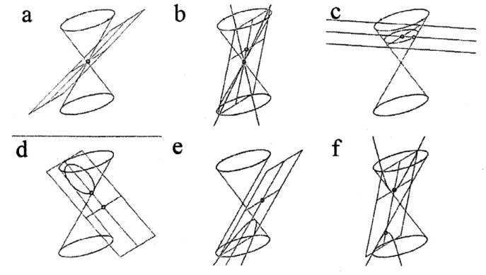
be beautifullyvisualized with colorful, interactive Cinderella[3] created Java applets.

Suitable exported applets allow to freely manipulate the position and orientation of the

plane inspace (comp. Fig. 1)$.[4,5,6]$ _{Cinderella’s}Spherical view (acentral ball projection

to the surface of

a

ball) allows

even

to visualize what happens at infinity. In this view it is

seen

that parabolas close at infinity, but hyperbolas remain divergent.

2.2

The

semi-latus

rectum

formula

A wellknown formula for the unified analytic description ofellipses, parabolas and

hyper-bolas is the semi-latus rectum $fo$ rmula. The radial distance $|\mathrm{r}|$ of

a

point

on

a

conic

curve

from a focus point in the direction of$\hat{\mathrm{r}}$ $-/$ $|\mathrm{r}|$ is given by

$| \mathrm{r}|=\frac{l}{1+c*\hat{\mathrm{r}}}$, (1)

where the semi-latus rectum is defined

as

the length ofthe excentricity vector

(perpen-dicular to the directrix, attached to the focus), times the length of the distance of the focus from the directrix

$l=|\epsilon$ $||\mathrm{d}|$ (2)

The asterisk product in eq. (1)

means

the scalar product of vectors. Depending

on

the scalar magnitude of the excentricity

we

obtain for

$\mathrm{o}$ $|\epsilon|<1$

an

ellipse, $\mathrm{o}$ $|\epsilon$ $|=1$

a

parabola,

82

a

$\sim$

$.’.’.\nearrow$

$\mathrm{b}$

$\iota_{1}$

$\overline{\backslash }\backslash ^{j}.\backslash \cdot\vee,.\nearrow’..\cdot.’$

..,

$\cdot$

$\mathrm{s}$

$.P’. \cdot...\cdot ^{’}\nearrow,\int_{j}$

$\nearrow,\cdot.\backslash _{\backslash _{\backslash }}\nearrow$

1

$J^{\cdot}.I_{\acute{}}\cdot..\cdot$,

$\mathrm{f}$

Figure 1: Conic (inter)sections: a) Point, b) pair ofintersecting straight lines, c) circle,

d) ellipse, e) parabola, f) hyperbola.

Thesemi-latus rectumformula

can

againbe colorfully visualized with

a

Cinderellacreated applet (compare Fig. 2)$.[4,5,6]$ It is possible to interactively change the directrix, the

focal

distance, the excentricity, and vary the radial direction by moving

a

point

on

the directrix. The semi-latus rectum $l$ appears

as

the distance between the focus,

and the intersection point of the conic section with

a

line parallel to the directrix through the focus. This happens precisely when the scalarproduct in eq. (1) vanishes, i.e. when $\hat{\mathrm{r}}$ is

parallel to the directrix.

2.3

Polar

angle description

of

ellipse

The polarangle parameter description

_of

an

ellipse is perhaps the most

common

descrip-tion of the ellipsestudied alreadyin highschool. Usually two mutuallyorthogonal vectors,

the semi-major axis vector

a

and the semi-minor axis vector $\mathrm{b}$ with

a

$*\mathrm{b}=0\Leftrightarrow$

a

1$\mathrm{b}$ (3)

are

linearly combined with trigonometric coefficients to give the distance of

a

point

on

the ellipse in the directionspecified by the polarangle _?

$\mathrm{r}=$

a

_{$\cos\varphi+$}$\mathrm{b}$_{$\sin\varphi$}

.

(4)

Cinderella created Java applets$[4, 6]$ both allow to

see

an animation with thepolar angle

$\varphi$

as

animation parameter, and

an

interactive version where the

two.

semi-axis, and the

83

$\mathrm{b}$ $\mathrm{c}$ $|\mathrm{i}$ , $——\cdot--.----..\cdot\cdot-\cdot-\cdot-.\cdot---$ . $:.\cdot.\acute{\mathit{1}}’..\cdot.-$

:.

. $J$ $’,\cdot.$

..

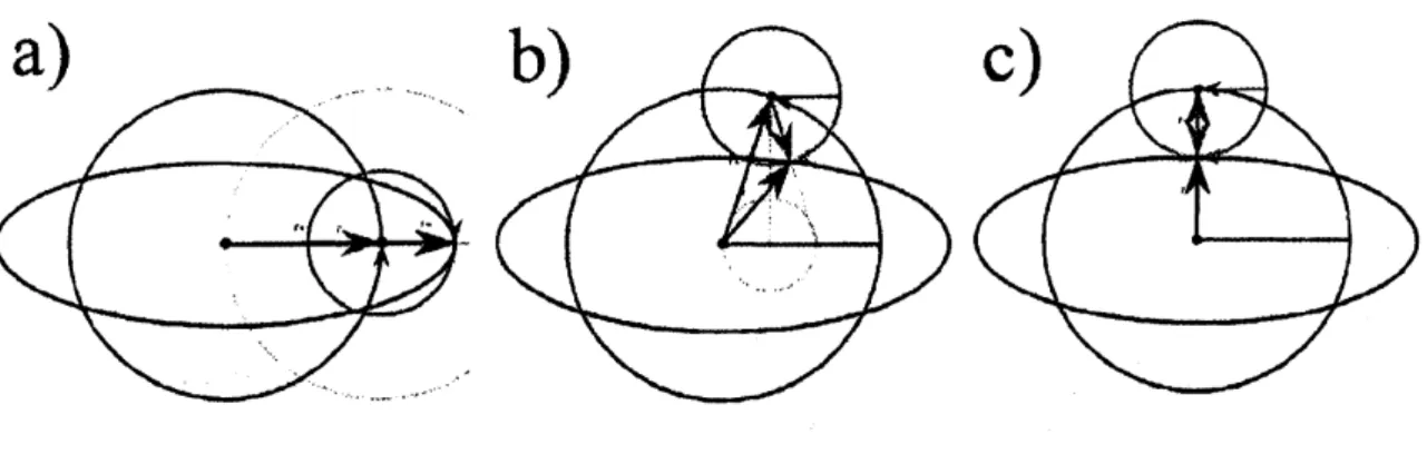
$\cdot$ -$.\cdot..\cdot.:\cdot\backslash .\cdot$ ., $|$

Figure 2: Semi-latus rectum formula: a) Ellipse, b) parabola, c) hyperbola.

c)

Figure 3: Polar angle parameter description

an

ellipse: a) polar angle in first quadrant,

94

a)

_,-...

_b)

_c)

. $\wedge$ $\cdot$ -$\cdot$

—–

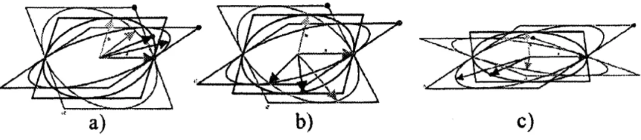
$\sim$ . $..\cdot.-\cdot’\backslash$ - – . .$J$

Figure4: Coplanar circular description of ellipse: a) $1=0$, b) $0<\varphi<\pi/2$, c) $\varphi=\pi/2$

.

2.4

Coplanar

circle

description

of

ellipse

The description of

an

ellipse by

means

of

a

linear combination oftwo circular motions in

one

plane (coplanar) is very instructive. Especially engineering students learn in this way

an easy-tO-apply method for generatingelliptical motions from circular motions:

$\mathrm{r}=\mathrm{r}_{+}+\mathrm{r}_{-}$, (5)

with the first circular motion in the unit bivector \’i-plane ofthe geometric algebra of the embedding vector space

$\mathrm{r}_{+}=\mathrm{r}_{+0}\exp(\mathrm{i}\varphi)$ (6)

and thesecond circular motion with opposite

sense

ofrotation in the

same

i-plane

$\mathrm{r}_{-}=\mathrm{r}_{-0}\exp(-\mathrm{i}\varphi)$

.

(7)

That forfixed$\mathrm{r}_{+0}$ and $\mathrm{r}_{-0}$ the trajectory of$\mathrm{r}$describes indeed

an

ellipse

can

beintuitively

illustrated with Cinderellacreated applets$[4, 6]$, both interactively (with free interactive

choices of$\mathrm{r}_{+0}$, $\mathrm{r}_{-0}$ and $\varphi$) and animated (compare Fig. 4).

2.5

Non-coplanar

circle

description of ellipse

It isfurtherpossibletodescribe

an

ellipse

as

a

linear combination oftwocircularmotions in

twoplanesofdifferent orientation (non-coplanar). The two circular motions

are

supposed

to have equal amplitude, frequency and phase. The twocircle planes

are

characterized in the geometric algebra of Euclidean threespace bytheirrespective unit bivectors $\mathrm{i}_{1}$ and $\mathrm{i}_{2}$.

That the planes

are

not coplanar means, that the intersection (or meet) will be

a

linear one-dimensional subspace represented by the vector

a

$=\alpha \mathrm{i}_{1}\vee \mathrm{i}_{2}=at$ $\mathrm{i}_{1}\llcorner(i\mathrm{i}_{1})$, (8)

where the symbol ” $\llcorner$” represents the right contraction [26] and $i$ the grade three

pseu-doscalarof the geometric algebra ofthree-dimensional Euclidean space. The real scalar$\alpha$

85

Figure 5: Non-coplanarcircle description ofellipse: a) $0<$ $\varphi$ $<\pi/2$, b) $3\pi/2$ $<p$ $<2\pi,$ c) changed orientation ofplanes.

the intersection of the two planes indicates rightly, that it will

serve as

the semi-major axis vector of the ellipse to be generated. The semi-minor axis vector will be

$\mathrm{b}=\frac{1}{2}\mathrm{a}(\mathrm{i}_{1}+\mathrm{i}_{2})$

.

(9)

The formula for the ellipse to be generated is

$\mathrm{r}=\frac{1}{2}\mathrm{a}\{\exp(10)+\exp(\mathrm{i}_{2}\varphi)\}$, $0\leq\varphi<2\pi.$ (10)

The ellipse generated according to (10)

can

be illustrated by interactive

or

animated

Cinderella created applets.$[4, 6]$ The intereactiveconstruction allows to change the length

of

a

and theindividual orientations of the planes. The dependence of the semi-minor axis

(9) on the two plane bivectors $\mathrm{i}_{1}$ and $\mathrm{i}_{2}$ is thus well visualized (compare Fig. 5).

2.6

Conic

sections

as

second

order

curves

Cinderella’s Locus mode is very suitable for visualizing the fact that conic sections

are

equivalent to second order

curves

according to the formula

$\mathrm{r}(\lambda)=\frac{\mathrm{a}_{0}+\mathrm{a}_{1}\lambda+\mathrm{a}_{2}\lambda^{2}}{\alpha+\lambda^{2}}$, (11)

with the vectors $\mathrm{a}_{0}$,$\mathrm{a}_{1}$,$\mathrm{a}_{2}$

.

The values of the real scalar $\alpha$ decide wether the resulting

quadratic

curve

is for

0 $\alpha>0$ an ellipse,

$\circ$ $\alpha=0$

a

parabola

or

0 $\alpha<0$

a

hyperbola.

The real scalar A parametrizes the

curves.

Interactive

Cinderella

created applets$[4, 6]$

allow to freely vary the vectors $\mathrm{a}\mathrm{o}$,

$\mathrm{a}_{1}$,$\mathrm{a}_{2}$ andthe scalars $\alpha$and A. One kind of animation

allows to show how the

curves

a

swept out by the vector $\mathrm{r}$ of

$\mathrm{e}\mathrm{q}\mathrm{u}$

.

(11) with A

as

the

ee

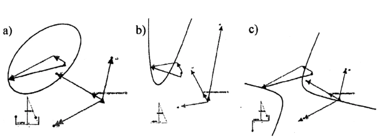
a) b) $\dot{}.\backslash \backslash$ $\cdot$ – $\sim.\cdot...\backslash$ -$\cdot\cdot$ $.\lrcorner$ $.\sim\ldots\backslash$

Figure 6: Conic sections

are

second order

curves:

a) $\alpha>0$ ellipse, b) $\alpha=0$ parabola,

c) $\alpha<0$ hyperbola. Apart from the complete curves, the graphs show the

vec-tors $\mathrm{a}_{0}$,$\mathrm{a}_{1}$,$\mathrm{a}_{2}$ and $\mathrm{a}$.linear combination of the three vectors with scalar coefficients

$\neg_{\alpha+\lambda}1\mathrm{g}$,$\neg_{\alpha+\lambda\alpha+\lambda}\lambda\lambda^{2}\mathrm{a}_{1,\neg}\mathrm{a}_{2}$ for

a

certain value of A.

3

Projective

description of plane

conic

sections

3,1

_{Pascal’s mystic}

_hexagon

Blaise Pascal (1623-1662, Fig. 7) researched the foundations ofhydrodynamics, stating that the pressure isthe

same

atallpointsin

a

fluid. Thisis the basis for hydraulic lifts. [27] But Pascal is also famous for his works in mathematics, both in theory and application.

He developed and sold e.g.

a

calculator machine. In his religious writings he famously

stated[28] :

If God does not exist,

one

will lose nothing by believing in him, while if he does exist,

one

will lose everything by not believing.

Our

present pointofinterest is Pascal’s work

on

conic sections.

At

the

age

of

16

he found what is

now

called “Pascal’s mystic hexagon”

or

less glamorous “Pascal’s theorem”:

If

a

hexagon (ABCDEX) isinscribed in

a

conic section, then the threepoints

($S_{1}$,$S_{2}$ and $\mathrm{S}_{3}$) where opposite side (lines) meet

are

collinear.[7]

The theorem is illustrated[7, 4, 6] in Fig. 8. The theorem is equally true for all plane

conic sections previously mentioned.

Formally speakingPascal’s theorem belongs to the field of“higher geometry,”

“geom-etry ofposition,” “descriptive geometry,”

or

in modern terms to “projective geometry.”

The six basic axioms of projective geometry

are

easy tounderstand[29]:

$\mathrm{o}$ If$A$ and $B$

are

distinct points

on a

plane, there is at least

one

line containing both

$A$ and $B$

.

$\mathrm{o}$ If$A$and $B$

are

distinctpoints

on a

plane, there is not

more

than

one

line containing

97

Figure 7: Blaise Pascal (1623-1662)[28]

38

Point $=$ Intersection oflines

$s_{1}$ $S_{2}$ $S_{3}$ $XA$ and $CD^{-}$ AB and DE $BC$ and $EX$

Table 1: Construction of$S_{1}$, $S_{2}$, and $S_{3}$

$\circ$ Any two lines in

a

plane have at least

one

point of the plane (which may be the

point at infinity) in

common.

$\mathrm{o}$ There is at least

one

line

on

a

plane.

$\mathrm{o}$ Every line contains at least three points oftheplane. $\mathrm{o}$ All the points of the plane do not belong to the

same

line.

3.2

Conic

sections

from

five points

Pascal’s construction of Fig. 8

can

be interpretedin twoimportant ways,

an

analytic and

a

constructive way. The analytic interpretation

was

given in the introduction.

The constructive interpretation

means

using the theorem for the construction of

a

conic section from five general points

on a

plane. Assume five points $A$,$B$,$C$,$D$,$E$ to

be given. Construct the four lines AB,$BC$,$CD$, DE and the point of intersection $S_{2}$

of the lines AB and DE. Next draw any line $g$ through the point $S_{2}$ and construct the

intersection points $S_{1}$ and$S_{3}$ ofthe line$\mathrm{g}$with $CD$ and $BC$, respectively. After thatdraw

the lines $S_{1}A$ and $S_{3}$E. According to Pascal’s theorem the point $X$ of intersection of the

lines$SiA$ and$S_{3}E$isalso

a

point

on

theconic section. By conducting this construction for

every angle ofthe line $g$ through the point 52, $X$ will sweep out the whole conic section.

This

can

be interactively realized with

a

Cinderellacreated applet.

A consequence is, that any point $X$ in the plane will be part of the conic section iff

it

can

be reached by changing the angle of line $g$ through point $S_{2}$. Therefore to decide

whether a point $X$ is

on

the conic section

or

not,

we

only need to check, whether Si, $S_{2}$,

and $S_{3}$

are

collinear (on

$g$)

or

not. The positions of$S_{1}$, and $S_{3}$ in this examination will

critically depend

on

the position of $X$ (compare Table 1).

3.3

Grassmann’s formula

Grassmann used precisely this method for obtaining his“equation of

a

conicsection that goes through the five points $A$,$B$,$C$,$D$,$E$,

no

three of which lie

on

the

same

straight

line”[8].

For this purpose he stated: “By planimetric multiplication I

mean

relative multipli-cation in the plane

as

a

domain of third order, ...”[8] This hint to the plane

as a

domain of third order is very important, because it shows that Grassmann actually expands the

plane projectively by adding

an

extradimension, commonly interpreted

as

the origin.

Grassmann further obtains the expression AB of

a

line from the outer product of

os

expression AB

comes

to

mean

both the product of two projective points $A$ and $B$ that

results in

an

algebraic representation of a line and the

common

symbolic representation

AB ofa line through two points $A$ and $B$.

Let us go into further geometric and algebraic details. The three-dimensional basis of

the projective space of

a

planeis given interms of three orthonormal vectors $\{\mathrm{e}_{1}, \mathrm{e}_{2}, \mathrm{e}_{0}\}$

.

The first two vectors span the familiar non-projective Euclidean plane. The third vector

$\mathrm{e}_{0}$, is the additional third dimension for liftingthe origin to $\mathrm{e}_{0}$. We represent a point in

the Euclidean plane by

a

linear combination of$\mathrm{e}_{1}$ and $\mathrm{e}_{2}$:

a

$=a_{1}\mathrm{e}_{1}+a_{2}\mathrm{e}_{2}$, (12)

where $a_{1}$ and $a_{2}$

are

simply the twO-dimensional

Cartesian

coordinates. The projective

representation[13] ofthe point $A$ is obtained by adding $\mathrm{e}_{0}$

$A=$

a

$+$$\mathrm{e}_{0}$

.

(13)

Projective points

are

homogeneous, i.e. $\lambda A$ represents the

same

point. The Euclidean

equivalent ofa projective point $A$ is obtained by

$\mathrm{a}=\frac{A-A*\mathrm{e}_{0}\mathrm{e}_{0}}{A*\mathrm{e}_{0}}$, (14)

I now deliberately introduce the product symbol ”$\Lambda$” for the exterior product in order to

ease

he distinction of thesymbolic representation of

a

lineAB and Grassmann’salgebraic

representation A$\Lambda B$. The exterior product is antisymmetric:

$A\wedge B=(\mathrm{a}+\mathrm{e}_{0})\wedge(\mathrm{b}+\mathrm{e}_{0})=$

a

$\Lambda \mathrm{b}+(\mathrm{a}-\mathrm{b})\Lambda \mathrm{e}_{0}$

.

(15)

a

$\Lambda \mathrm{b}$ is the moment bivector of

a

line and $(\mathrm{b}-\mathrm{a})$ is its direction vector. The two

entities suffice to construct the line.[ll] Grassmann’s planimetric product oftwolines AB andDE

can

be realizedin thegeometric algebra of the projective three-dimension$\mathrm{a}1$ space

spanned by $\{\mathrm{e}_{1}, \mathrm{e}_{2}, \mathrm{e}_{0}\}$ by

$S_{2}=(A\Lambda B)\llcorner$[I3$(D\Lambda E)$], (16)

where the symbol ” $\llcorner$” represents the right contraction[26] and $I_{3}=\mathrm{e}_{1}\Lambda \mathrm{e}_{2}\Lambda \mathrm{e}_{0}=\mathrm{i}\mathrm{e}_{0}$

is the volume 3-vector of the projective space ( $\mathrm{i}=\mathrm{e}_{1}\Lambda \mathrm{e}_{2}$ is the unit bivector of the

Euclidean plane spanned by$\mathrm{e}_{1}$ and$\mathrm{e}_{2}$)

.

$[I_{3}(D\Lambda E)]$ results inthedual complementvector

perpendicular to theprojective linebivector DAE. Finallythe right contraction with the line bivector $A$$\Lambda B$ results in the element $S_{2}$ in the line A$\Lambda B$, which isperpendicular to

[I3 ($D\Lambda E$)] in$A\wedge B$, andtherefore also contained in$D\Lambda E$. Inserting (13) andsimplifying

the expressions algebraically, weget for the intersection

$S_{2}=\lambda_{2}\mathrm{s}_{2}+\lambda_{2}\mathrm{e}_{0}=$ (a -b)$[\mathrm{i}(\mathrm{d}\wedge \mathrm{e})]-(\mathrm{d}-\mathrm{e})[\mathrm{i}(\mathrm{a}\Lambda \mathrm{b})]+\mathrm{i}[(\mathrm{d}-\mathrm{e})\Lambda(\mathrm{a}-\mathrm{b})]\mathrm{e}_{0}$ (17)

In projective geometry points

are

identical up to scalar factors. We therefore divide by

100

to get according to eq. (14) the plane Euclidean vector

$\mathrm{s}_{2}=\frac{1}{\lambda_{2}}\{(\mathrm{a}-\mathrm{b})[\mathrm{i}(\mathrm{d}\wedge \mathrm{e})]-(\mathrm{d}-\mathrm{e})[\mathrm{i}(\mathrm{a}\wedge \mathrm{b})]\}$ (19)

Inserting coordinates (13)

we

explicitly get

$\mathrm{s}_{2}=\frac{1}{\lambda_{2}}\{(d_{1}e_{2}-d_{2}e_{1})(\mathrm{a}-\mathrm{b})-(a_{1}b_{2}-a_{2}b_{1})(\mathrm{d}-\mathrm{e})\}$ (20)

In the very

same

way Grassmann calculates $S_{1}$ and $S_{3}$ by planimetric products

as

$S_{1}=(X\Lambda A)\mathrm{L}$[I3$(C$$\Lambda D)$], $S_{\theta}=(B\Lambda C)\mathrm{L}$[I3(D$\wedge X)$], (21)

So

we can

finallyexpress the collinearity of Si, $S_{2}$ and $S_{3}$ by

$S_{1}\Lambda S_{2}\wedge S_{3}=0,$ (22)

i.e.

$\{(X\wedge 4)\llcorner[I_{3}(C\Lambda D)]\}\Lambda$

{

$(A\wedge B)\llcorner$[I3$(D\Lambda E)]$

}

$\Lambda$

{

_{$(B\Lambda C)\llcorner$}[I3$(E\wedge X)]$

}

$=0.$ (23)

ThisisGrassmann’s formula for the conic sections throughfivegeneralpoints $(A,$$B$,$C$,$D$, $E)$ in

a

planeexpressed inthe geometric algebra of the projective space$\{\mathrm{e}_{1}, \mathrm{e}_{2}, \mathrm{e}_{0}\}$

.

Every

point $X$, that fulfills equation (23) will be onthe conic section. The equation is quadratic

in $X$ and in all ofthefivepoints$A$,$B$,$C$,$D$,$E$

.

Withthe helpoftheanticommutator”$\mathrm{x}$”

$B_{1} \mathrm{x}B_{2}=\frac{1}{2}$(_{$B_{1}B_{2}-$} B2BX) (24)

we

can

rewrite (23)

as

$\{[(X\wedge 4)\mathrm{x}(C\wedge D)]\mathrm{x}[(A\wedge B)\mathrm{x}(D\Lambda E)]\}\Lambda\{I_{\theta}[(B\wedge C)\mathrm{x}(E\wedge X)]\}=0.$ (25)

4

Conformal

geometric

algebra description of

plane

conic

sections

4,1

_{Grassmann’s formula for the conformal model}

The

five-dimensional

conformal model [10, 11, 12, 13, 14] adds to the three-dimensional Euclidean space twodimensions:

one

for representing the origin and

one

for representing infinity. This is done by introducing two null-vectors, which square to

zero

and

are

perpendicular to thevectors ofEuclidean space:

$\{\overline{\mathrm{n}}, \mathrm{e}_{1}, \mathrm{e}_{2}, \mathrm{e}_{3}, \mathrm{n}\}$, (20)

where$\overline{\mathrm{n}}$and

$\mathrm{n}$representtheorigin andinfinity, respectively. Theconformalrepresentation

of

a

point $A$ is obtained by adding two contributions

101

with $a^{2}=$

aa.

A straight Euclidean line AB in the conformal model is given bythe outer

product of wo points

on

the line with infinity forming the trivector

$A$$\Lambda B\Lambda \mathrm{n}=$ a$\Lambda \mathrm{b}\wedge \mathrm{n}+(\mathrm{b}-\mathrm{a})N=\mathrm{m}_{\mathrm{l}}\mathrm{n}+\mathrm{d}_{1}N$, (28)

where the unit bivector$N=\mathrm{n}\Lambda\overline{\mathrm{n}}$represents the additionaltwo dimensional (Minkowski)

space. A point $X$ is

on

the line AB iff

$X\Lambda$A$\Lambda B\Lambda \mathrm{n}=0.$ (29)

Similarly the line DE is given by the trivector

$D\Lambda E\wedge \mathrm{n}=\mathrm{d}\Lambda \mathrm{e}\Lambda \mathrm{n}+(\mathrm{e}-\mathrm{d})N=\mathrm{m}_{2}\mathrm{n}+\mathrm{d}_{2}N$, (30)

where $\mathrm{m}_{1}$ and $\mathrm{m}_{2}$

are

the Euclidean moment bivectors of the lines AB and DE, and the

vectors $\mathrm{d}_{1}$ and $\mathrm{d}_{2}$ aretheir directionvectors, respectively. Theintersection$S_{2}^{c}$oftwo lines

AB and DE is obtained in

a

fashion very similar to (16)

$S_{2}^{c}\wedge \mathrm{n}=(A\wedge B\wedge \mathrm{n})\llcorner[I_{4}(D\Lambda E\wedge \mathrm{n})]$ , $S_{2}^{c2}=0,$ (31)

where $I_{4}=$ iN, with \’ibeing the bivector that represents the plane shared by $A$,$B$,$D$ and $E$

.

We

now

perform

a

detailed calculation of the rightside ofthe first equation of(31) in

order to show that the specialform ofthe bivector on the left side is indeed justified. (A

reader less familiar with geometric algebra may skip this calculation.)

$(A\wedge B\Lambda \mathrm{n})\mathrm{L}[I_{4}(D\wedge E\Lambda \mathrm{n})]=$ $(30)$ $+\mathrm{d}_{1}N)\mathrm{i}N(\mathrm{m}_{2}\mathrm{n}+\mathrm{d}_{2}N)\rangle_{2}$

$=\langle \mathrm{m}_{1}\mathrm{n}\mathrm{i}N\mathrm{m}_{2}\mathrm{n}+\mathrm{m}_{1}\mathrm{n}\mathrm{i}N\mathrm{d}_{2}N+$

dlNiNm2n

$+\mathrm{d}_{1}N\mathrm{i}N\mathrm{d}_{2}N\rangle_{2}$

$=\langle \mathrm{i}\mathrm{m}_{\mathrm{l}}\mathrm{n}7\mathrm{V}\mathrm{n}\mathrm{m}_{2}+\mathrm{i}\mathrm{m}_{1}\mathrm{n}\mathrm{d}_{2}N+\mathrm{d}\mathrm{i}\mathrm{i}\mathrm{m}2\mathrm{n}+\mathrm{d}_{1}\mathrm{i}\mathrm{d}_{2}N\rangle_{2}$

$=\langle 0-$ imid2n$+$im2din$+\mathrm{i}\mathrm{d}_{1}\mathrm{d}_{2}\overline{\mathrm{n}}\wedge \mathrm{n}\rangle_{2}$ $=\langle--\mathrm{i}\mathrm{r}\mathrm{o}_{1}\mathrm{d}_{2}+\mathrm{i}\mathrm{m}2\mathrm{d}\mathrm{i}\mathrm{n}\langle \mathrm{i}\mathrm{d}_{1}\mathrm{d}_{2}\rangle_{0}\mathrm{i})_{1}$ $\wedge$n.

$\lambda_{2}\mathrm{s}_{2}$ -A2 (32) (33) (34) (35) (36)

Angularbrackets with

an

integer grade index ( $\rangle_{k}$,$k\geq 0$ referto theoperationofgrade $k$

selection. The equality in (32) is

a

simple applicationof the definition of the contraction of

a

vector $\mathrm{I}\mathrm{A}(\mathrm{D}\Lambda E\Lambda \mathrm{n})$ (_$=$ the dual of the trivector $(D\Lambda E\Lambda \mathrm{n})$) from the rightonto

a

trivector to the left.[26] The equality between lines (33) and (34)

uses

the following identities: $\mathrm{m}_{1}\mathrm{n}\mathrm{i}=$ imin, $\mathrm{m}_{2}\mathrm{n}=\mathrm{n}\mathrm{m}_{2}$, $N\mathrm{i}=\mathrm{i}N=I_{4}$, and $NN=1.$ The equality

between the lines (34) and (35)

uses

the following identities: $\mathrm{n}N=$ n,

nn

$=0,$ and

hence $\mathrm{n}N\mathrm{n}=0.$ It further

uses

$\mathrm{n}\mathrm{d}_{2}=-\mathrm{d}_{2}\mathrm{n}$, $\mathrm{d}_{1}\mathrm{i}=-\mathrm{i}\mathrm{d}\mathrm{i}$, $\mathrm{d}_{1}\mathrm{m}_{2}=-\mathrm{m}_{2}\mathrm{d}_{1}$, and that

$N=\mathrm{n}\Lambda \mathrm{i}$ $=-$ $\mathrm{i}$$\Lambda \mathrm{n}$ is already a bivector. It remains to be observed that in line (36)

the entities $\mathrm{i}\mathrm{m}_{1}$, $\mathrm{i}\mathrm{m}_{2}$ and $\langle \mathrm{i}\mathrm{d}_{1}\mathrm{d}_{2}\rangle_{0}=-\lambda_{2}$

are

all scalars, whereas

$\mathrm{d}\mathrm{i}$,

$\mathrm{d}_{2}$ and $\mathrm{i}$

are

all

vectors.

The explicit calculation of (31) yields therefore

102

with the

same

Euclidean vector $\mathrm{s}_{2}$

as

in equations (19) and (20). Note that $\mathrm{n}\wedge \mathrm{n}=0,$

but the term $(s_{2}^{2}/2)\mathrm{n}$isinserted to fulfill $S_{2}^{c2}=0,$ the secondpart of(31). Similar to (31)

weobtain

$S_{1}^{c}\wedge \mathrm{n}=(X\wedge A \Lambda \mathrm{n})$ $\llcorner[I_{4}(C\wedge D\wedge \mathrm{n})]$, $S_{1}^{c2}=0,$ (38)

and

$S_{3}^{c}\Lambda \mathrm{n}=(B\Lambda C\Lambda \mathrm{n})\mathrm{L}[\mathrm{h}\{\mathrm{E}\wedge X\wedge \mathrm{n})]$, $S_{3}^{c2}=0.$ (39)

Using the three

conformal

points of intersection $S_{1}^{c}$, $S_{2}^{c}$ and $S_{3}^{c}$

we

can

finally give the

equation for the

conic

sections through five general points

on

a

plane in the conformal model

as

$S_{1}^{c}\Lambda S_{2}^{c}\Lambda S_{3}^{c}\Lambda \mathrm{n}=0.$ (40)

Thisis the conformal equivalent of Grassmann’s formulaforconicsections, which in turn has been

seen

to be based

on

Pascal’s theorem. Every conformal point$X=x+\mathrm{j}x^{2}$ $\mathrm{i}+\mathrm{n}$

that fulfills (40) is

on

the plane conic section through $A$,$B$,$C$,$D$,$E$

.

By construction,

equation (40) is again quadratic in $X$ and in all of the five points $A$,$B$,$C$,$D$,$E$

.

4.2

Cirlces

This quadratic property of(40) is in contrast to the simpler representation ofcircles[ll]

by three conformal points $A_{1}$, $A_{2}$ and

A3

$A_{1}\Lambda A_{2}\Lambda 4_{3}$

.

(41)

According to (28) straight lines

are

simplycircles through infinity $\mathrm{n}$

.

All points$\mathrm{X}$

on

the

circle through $A_{1}$, $A_{2}$ and

A3

are simply obtained from

$X\wedge A_{1}\wedge A_{2}\wedge A_{3}=0.$ (42)

This equation is linear in $\mathrm{X}$ and in the three general defining points

$A_{1}$, $A_{2}$ and

A3.

The

explicit form of(41) becomes

$\frac{1}{2}(a_{1}^{2}\mathrm{a}_{2}\Lambda \mathrm{a}_{3}+a_{2}^{2}\mathrm{a}_{3}\Lambda \mathrm{a}_{1}+a_{3}^{2}\mathrm{a}_{1}\Lambda \mathrm{a}_{2})\mathrm{n}$

$+(\mathrm{a}_{3} \Lambda \mathrm{a}_{1}+\mathrm{a}_{2}\wedge \mathrm{a}_{3}+\mathrm{a}_{1}\Lambda \mathrm{a}_{2})\mathrm{n}-$ (43)

$+ \frac{1}{2}([a_{2}^{2}-a_{3}^{2}]\mathrm{a}_{1}+[a_{3}^{2}- a_{1}^{2}]\mathrm{a}_{2}+[a_{1}^{2}-a_{2}^{2}]\mathrm{a}_{3})N$

.

The expected first term $\mathrm{a}_{1}\Lambda \mathrm{a}_{2}\wedge \mathrm{a}_{3}$ will be zero, because

we

assume a

circle in two

Euclidean

dimensions2

and not three, i.e. the origin $\mathrm{i}$ will always be in the circleplane.

Separatingoff the circle center vector $\mathrm{c}$ and the radius $r(x_{1}^{2}=x_{2}^{2}=x_{3}^{2}=1)$

$\mathrm{a}_{1}=\mathrm{c}+r\mathrm{x}_{1}$, $\mathrm{a}_{2}=\mathrm{c}+r\mathrm{x}_{2}$

,

a3 $=\mathrm{c}+r\mathrm{x}_{3}$, (44)

we

finally get for (43)

$\mathrm{c}(\mathrm{c}\wedge I_{c})\mathrm{n}+\frac{1}{2}(r^{2}-c^{2})I_{\mathrm{c}}\mathrm{n}+I_{\mathrm{c}}\overline{\mathrm{n}}-\mathrm{c}I_{\mathrm{c}}N$, (45)

$2\mathrm{A}$more general

103

where

we

set the bivector of the circleplain to

$I_{c}=(\mathrm{a}_{3}-\mathrm{a}_{2})\Lambda(\mathrm{a}_{1}-\mathrm{a}_{2})$. (46)

Because

we

assume, that

we

are

just dealing with the plane two dimensional

case

the circle center $\mathrm{c}$ must also be in the $I_{c}$-plane (i.e. $c\Lambda I_{c}=0$) and hence

$A_{1}\wedge A_{2}\wedge A3$ $=$ [$\frac{1}{2}(r^{2}-c^{2})\mathrm{n}+\overline{\mathrm{n}}-$cN]Ic. (47)

We therefore

see

how (41) includescomponentbycomponentthecircleplane$I_{e}$, thecenter

$\mathrm{c}$ and the radius $r$. Equation (42) is

a

condition for all points $X$

on

the circle (41). By

inserting $X= \mathrm{x}+\frac{1}{2}x^{2}\mathrm{n}+\overline{\mathrm{n}}$ into (42) we get after

some

algebra

$(\mathrm{x}-\mathrm{c})^{2}=r^{2}$

.

(48)

Acknowledgements

Theheavens declare thegloryofGod; the skiesproclaimthe work of his hands. Day afterdaytheypour forth speech; nightafter night theydisplay knowledge. There is

no

speech

or

language where their voice is not heard. Their voice

goes

out into all the earth, their words to the ends of the world.[30]

I thank my dear wife and my dear sons,

as

well as H. Ishi, R. Nagaoka and J. Browne. Soli Deo Gloria.

References

[1] P. Lounesto, Clifford Algebras and Spinors, CUP, Cambridge, 2001.

homepage mirror: $<$http://www.hut.fi/ $\mathrm{p}\mathrm{p}\mathrm{u}\mathrm{s}\mathrm{k}\mathrm{a}/\mathrm{m}\mathrm{i}\mathrm{r}\mathrm{r}\mathrm{o}\mathrm{r}/\mathrm{L}\mathrm{o}\mathrm{u}\mathrm{n}\mathrm{e}\mathrm{s}\mathrm{t}\mathrm{o}/>$

[2] D. Hestenes, New Foundations for Classical Mechanics (2nd ed.), Kluwer,

1999.

[3] Cinderellawebsite $<$http://www.cinderella.de/en/home/index.html$>$,

Cinderella Japan website $<$http://www.cinderella.de/en/home/index.html$>$

[4] E. Hitzer, $<$http:$//\mathrm{s}\mathrm{i}\mathrm{n}\mathrm{a}\mathrm{i}$.mech.fukui-u.ac.j$\mathrm{p}/\mathrm{g}\mathrm{c}\mathrm{j}/\mathrm{s}\mathrm{o}\mathrm{f}\mathrm{t}\mathrm{w}\mathrm{a}\mathrm{r}\mathrm{e}/\mathrm{G}\mathrm{A}\mathrm{c}\mathrm{i}\mathrm{n}\mathrm{d}\mathrm{y}/\mathrm{G}\mathrm{A}\mathrm{c}\mathrm{i}\mathrm{n}\mathrm{d}\mathrm{y}$ .htm$>$

$[5]$ E. Hitzer, UAJ LA2 support website

http:$//\mathrm{s}\mathrm{i}\mathrm{n}\mathrm{a}\mathrm{i}$.mech.fukui-u.$\mathrm{a}\mathrm{c}.\mathrm{j}\mathrm{p}/\mathrm{g}\mathrm{a}\mathrm{l}\mathrm{a}2/\mathrm{i}\mathrm{n}\mathrm{d}\mathrm{e}\mathrm{x}$.html

[6] E. Hitzer, Presentation at Innovative Teaching

_of

Mathematics with Geometric

Al-gebra 2003, Nov. 20-22, Kyoto University, Japan.

http: //sinai.mech.fukui-u.ac.jp[ITM2003/

presentations/Hitzer’

pagel.html [7] World website, $\mathrm{h}\mathrm{t}\mathrm{t}\mathrm{p}://\mathrm{m}\mathrm{a}\mathrm{t}\mathrm{h}\mathrm{w}\mathrm{o}\mathrm{r}\mathrm{l}\mathrm{d}.\mathrm{w}\mathrm{o}\mathrm{l}\mathrm{f}\mathrm{r}\mathrm{a}\mathrm{m}.\mathrm{c}\mathrm{o}\mathrm{m}/\mathrm{P}\mathrm{a}\mathrm{s}\mathrm{c}\mathrm{a}\mathrm{l}\mathrm{s}\mathrm{T}\mathrm{h}\mathrm{e}\mathrm{o}\mathrm{r}\mathrm{e}\mathrm{m}.\mathrm{h}\mathrm{t}\mathrm{m}\mathrm{l}$

[8] H. Grassmann, Extension Theory, $\mathrm{t}\mathrm{r}$

.

by L. Kannenberg, AMS, Hist, ofMath., 2000.

104

[10] D. Hestenes, H. Li, A. Rockwood in G. Sommer (ed.) Geometric Computing with

Cliff. Alg., Springer, 2001.

[11] E. Hitzer, KamiWaAi- Interactive $3\mathrm{D}$ Sketching with Java based

on

Cl$(4,1)$

Confor-mal Model of Euclidean Space, Adv. in Ap. Clif. Alg. 13(1) pp. 11-45 (2003).

http://sinai.mech.fukui-u.$\mathrm{a}\mathrm{c}.\mathrm{j}\mathrm{p}/\mathrm{g}\mathrm{c}\mathrm{j}/$publications/KWAdoc/KWAdcibs.html

[12] E. Hitzer, Homogeneous Model of Euclidean Space in theCl$(4,1)$ Algebra of

{origin,

3-space,

infinity}

and Java ImpL, lect. at ICIAM Clif. Minisymp., Sydney 2003. [13] C. Doran, A. Lasenby, J. Lasenby Conformal Geometry, Euclidean Space and

GeO-metric Algebra, in J. Winkler (ed.), Uncertainty in Geom. Comp., Kluwer, 2002.

[14] L. Dorst, Interactively Exploring the Conformal Model, Lecture at Inn. Teach,

_of

Math, _{with Geometric Algebra 2003, Nov. 20-22, Kyoto University, Japan.}

[15] H. Grassmann, A

new

branch ofMath., $\mathrm{t}\mathrm{r}$

.

by L. Kannenberg, Open Court, 1995.

[16] A. Beutelspacher in G. Schubring (ed.), $\mathrm{H}.\mathrm{G}$. Grassmann, Kluwer, Dordrecht,

1996.

[17] W. K. Clifford. Appl. of Grassmann’s extensive algebra.

Am. J.

Math., 1:350,

1878.

[18] J. Browne, $<$http://www.ses.swin.edu.au/homes/browne$/\mathrm{i}\mathrm{n}\mathrm{d}\mathrm{e}\mathrm{x}.\mathrm{h}\mathrm{t}\mathrm{m}>$

[19] W. R. HamiltonOn

a

newSpeciesofImag. Quant, connected$\mathrm{w}$

.

a

th.ofQuaternions,

Proc. ofRoy. Irish Acad., Nov. 13, 1843, 2, 424-434.

[20] D. Hestenes, G. Sobczyk, Clifford Algebra to Geometric Calculus, Kluwer, 1992.

[21] C. Doran, L. Dorst and J. Lasenby $\mathrm{e}\mathrm{d}\mathrm{s}.$, Appl. Geom. Alg. in Comp. Science and

Engineering, AGACSE 2001, Birkhauser, 2002.

[22] E. Hitzer, Geometric Calculus-Engineering Mathematics for the21stCentury, Mem.

Fac. Eng. Fukui Univ. 50(1), 2002.

[23]

G.

Sobczyk,

Clifford Geometric

Algebras in Multilinear Algebraand Non-Euclidean Geometries, Lecture at Comp. Noncom. Algebra and AppL, July 6-19, 2003,

$\mathrm{h}\mathrm{t}\mathrm{t}\mathrm{p}://\mathrm{w}\mathrm{w}\mathrm{w}$.prometheus-inc.$\mathrm{c}\mathrm{o}\mathrm{m}/\mathrm{a}s\mathrm{i}/\mathrm{a}\mathrm{l}\mathrm{g}\mathrm{e}\mathrm{b}\mathrm{r}\mathrm{a}2003/\mathrm{a}\mathrm{b}\mathrm{s}\mathrm{t}\mathrm{r}\mathrm{a}\mathrm{c}\mathrm{t}\mathrm{s}/\mathrm{s}\mathrm{o}\mathrm{b}\mathrm{c}\mathrm{z}\mathrm{y}\mathrm{k}$.pdf

[24] L. Dorst, GAViewer website $<\mathrm{h}\mathrm{t}\mathrm{t}\mathrm{p}://\mathrm{w}\mathrm{w}\mathrm{w}.\mathrm{s}\mathrm{c}\mathrm{i}\mathrm{e}\mathrm{n}\mathrm{c}\mathrm{e}.\mathrm{u}\mathrm{v}\mathrm{a}.\mathrm{n}\mathrm{l}/\mathrm{g}\mathrm{a}/\mathrm{v}\mathrm{i}\mathrm{e}\mathrm{w}\mathrm{e}\mathrm{r}/>$

[25] C. Perwass, CLUCalc website, $<$http:[/www.perwass.de/cbup$\oint$clu.html>

[26] L. Dorst, The Inner Products ofGeometric Algebra,

in

L. Dorst et. al. $(\mathrm{e}\mathrm{d}\mathrm{s}.)$,

Appli-cations ofGeometric Algebrain Comp. Sc. and Eng., Birkhaeuser, Basel, 2002.

[27] Science World website: Pascal biography entry,

http:[$/\mathrm{s}\mathrm{c}\mathrm{i}\mathrm{e}\mathrm{n}\mathrm{c}\mathrm{e}\mathrm{w}\mathrm{o}\mathrm{r}\mathrm{l}\mathrm{d}$.wolfram.$\mathrm{c}\mathrm{o}\mathrm{m}/\mathrm{b}\mathrm{i}\mathrm{o}\mathrm{g}\mathrm{r}\mathrm{a}\mathrm{p}\mathrm{h}\mathrm{y}/\mathrm{P}\mathrm{a}\mathrm{s}\mathrm{c}\mathrm{a}\mathrm{l}$.html

[28] $\mathrm{h}\mathrm{t}\mathrm{t}\mathrm{p}://\mathrm{w}\mathrm{w}\mathrm{w}$

-groups.

$\mathrm{d}\mathrm{c}\mathrm{s}.\mathrm{s}\mathrm{t}$-and.

$\mathrm{a}\mathrm{c}.\mathrm{u}\mathrm{k}/\mathrm{h}\mathrm{i}\mathrm{s}\mathrm{t}\mathrm{o}\mathrm{r}\mathrm{y}/\mathrm{M}\mathrm{a}\mathrm{t}\mathrm{h}\mathrm{e}\mathrm{m}\mathrm{a}\mathrm{t}\mathrm{i}\mathrm{c}\mathrm{i}\mathrm{a}\mathrm{n}\mathrm{s}/\mathrm{P}\mathrm{a}\mathrm{s}\mathrm{c}\mathrm{a}\mathrm{l}$.html

[29] O. Veblen, J. Young, Projective Geometry, 2 vols. Boston, MA: Ginn,

1938.