JAIST Repository
https://dspace.jaist.ac.jp/Title Automatic Generation Method for Processing Plants
Author(s) Nomura, Kentarou; Miyata, Kazunori
Citation Forma, 26(1): 29-38
Issue Date 2011
Type Journal Article
Text version author
URL http://hdl.handle.net/10119/10681
Rights Copyright (C) 2011 形の科学会. Kentarou Nomura,
Kazunori Miyata, Forma, 26(1), 2011, 29-38. Description
Category:
Original Paper
Title:
Automatic Generation Method for Processing Plants
Authors:
Kentaro NOMURA and Kazunori MIYATA
Affiliations:
Japan Advanced Institute of Science and Technology, [email protected]
Keywords:
Procedural Modeling, Processing Plant, Geometry Model
Abstract
A processing plant consists of massive parts including tanks, pipelines, processing columns, frames, and so on. This paper reports a method for automatically generating the landscape of a processing plant from a 2D sketch input and some control parameters. This is difficult to implement with conventional procedural methods. The results show that the landscapes of a processing plant are satisfactorily represented, while some detailed parts, such as valves, steps, and branching pipelines, are not generated. The generated 3D geometric data are useful for constructing background scenes in movies and video games, and are also applicable for pre-visualizing a landscape to construct a processing plant.
1. Introduction
This paper proposes a method for automatically generating the landscape of a processing plant from a 2D sketch input, which is difficult to implement with conventional procedural methods. The generated 3D geometric data are useful for constructing background scenes in movies and video games, and are also applicable for pre-visualizing a landscape to construct a processing plant.
1.1 Background
Recently, massive geometric models, such as buildings and forests, are required to produce high-definition computer-generated imagery. The accuracy and the volume of the models are increasing, and consequently the workload in the modeling process becomes heavier. It is therefore important to generate contents procedurally or automatically, so as to produce such models efficiently.
The main target of this paper is processing plants. A processing plant consists of massive parts, and most of the parts are connected to other parts with pipelines. It is very hard to assemble such complicated geometric models manually. Our method can generate the landscape of a processing plant from a 2D sketch input which specifies the outline of an intended model. We do not pursue precision in the functionality of the processing plant, but consider visual satisfaction.
1.2 Related works
Grammar-based modeling covers many targets, from generation of natural shapes to architectural models. Procedural Inc. sells software, CityEngine (Procedural Inc., 2008), for generating a large-scale 3D urban environment procedurally, including street networks and 3D buildings. Frischer et al. have applied this software to rebuild highly-detailed ancient Rome at the peak of the Roman Empire (Frischer, 2008). However, this software does not consider connectivity of buildings.
Parish and Müller proposed a system using a procedural approach based on L-system to model virtual cities (Parish and Müller, 2001). Müller et al. reported a novel shape grammar, CGA shape, for the procedural modeling of building shells to obtain large scale city models (Müller et al., 2006). They also introduced algorithms to automatically derive 3D models of high visual quality from single facade images of arbitrary resolutions (Müller et al., 2007).Shape Grammar (Stiny, 1980) and Split Grammars (Wonka et al., 2003) are also used for shape, facade and detail modeling.There are automatic generation methods using a model input by a user, to generate a large complex model that resembles the user input (Merrell, 2007; Merrell and Manocha, 2009). These approaches are extensions of texture synthesis based on 3D geometry. There are also ways of combining procedural methods and interactive editing. In (Chen et al., 2008), users can create a street network or modify an existing street network by editing an underlying tensor field.
Most of these procedural methods generate virtual cites from two-dimensional images. In contrast, this paper proposes a method to generate a processing plant model which consists of tanks and pipes from two-dimensional sketch input.
Fujita et al. presented a constraint-directed approach for layout design of power plants by representing conditions as spatial constraints (Fujita et al., 1992). In their method, the user has to specify the parts to be placed and constraint conditions of a power plant. However, it is not easy for a user who does not have any knowledge about power plants to input technical data. In our method, a user can design a process plant intuitively by drawing 2D sketch input.
2. Overview of a Processing Plant
A processing plant consists of massive and interlacing parts including tanks, pipelines, processing columns, frames, and so on as shown in Fig. 1(see also Ohyama and Ishii, 2007). In the real world, a plant layout is designed considering the space, relations between parts, material handling, communications, utilities, and structural forms. The main purpose of this paper is to generate the landscape of a processing plant from simple input data, so we only consider the space and structural forms of the plant, and do not care about the precise details of functionality. Therefore, our method generates only towers, pipelines, tanks, and frames. Other apparatus, such as valves, flarestacks, lights, and ladders are not considered, because these models are so small compared with towers and tanks.
3. Generation Method for Processing Plant
This section describes the overview of the algorithm, and then explains each process in detail. 3.1 Process Overview
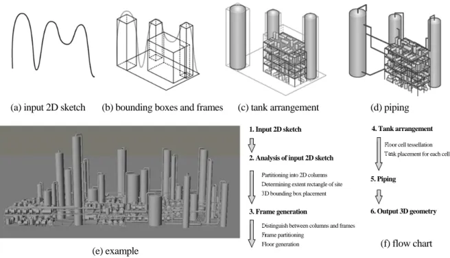
Our algorithm for generating a processing plant model consists of the following four steps, which are also illustrated in Fig.2;
(1) Analysis of 2D sketch input
(2) Frame generation from the bounding boxes (3) Tank arrangement
(4) Piping
The procedure first analyses 2D sketch input. Here, a 2D sketch specifies the profile of a processing plant. Then 3D bounding boxes are generated from the 2D sketch. Next, frames are generated from the bounding boxes, then tanks are arranged on each floor. Finally, each tank is connected to adjoining tanks by pipelines.
#1: (a) Tower, (b) Frame, (c) Pipeline #2: (a) Tank, (b) Frame, (c) Pipeline
Figure 1: Example of Processing Plant ( courtesy of http://www.photolibrary.jp/)
(a) (b) (c) (a) (c) (b)
3.2 Analysis of Input 2D Sketch
3D bounding boxes of the processing plant are generated from a 2D sketch which is drawn with a single stroke.
First, the input 2D sketch is partitioned into columns as shown in Fig. 3. The specified 2D sketch is scanned from left to right to calculate the gradient of the profile, dy/dx. A column is formed when the absolute value of the gradient is over the pre-defined threshold parameter. The steeper the gradient, the narrower the width. Here, the minimum column width is also pre-defined. We have set the threshold parameter to 0.9, and the minimum width to 15, respectively. If there is an overhang in the 2D sketch as shown in Fig. 4 (a), the relevant curve is flattened as shown in Fig. 4 (b) by connecting the start point, Ps, and the end point, Pe, with a straight line.
Then, the extent rectangle of the site for the processing plant is determined by placing the 2D sketch so as to fit the diagonal of the rectangle as shown in Fig. 5(a). Here, the three-dimensional viewing angle is specified by a user. Next, a bounding box for each column is placed randomly within the obtained extent rectangle of the site, by sliding its position according to the viewing direction, as shown in Fig. 5(b).
(e) example
Figure 2: Procedure Overview
(a) input 2D sketch (b) bounding boxes and frames (c) tank arrangement (d) piping
1. Input 2D sketch
2. Analysis of input 2D sketch
Partitioning into 2D columns Determining extent rectangle of site 3D bounding box placement
3. Frame generation
Distinguish between columns and frames Frame partitioning
Floor generation
4. Tank arrangement
5. Piping
6. Output 3D geometry
Floor cell tessellation Tank placement for each cell
(f) flow chart
Figure 3: Partitioning of 2D Sketch Figure 4: Processing for overhang
Ps Ps
Pe Pe
3.3 Frame Generation
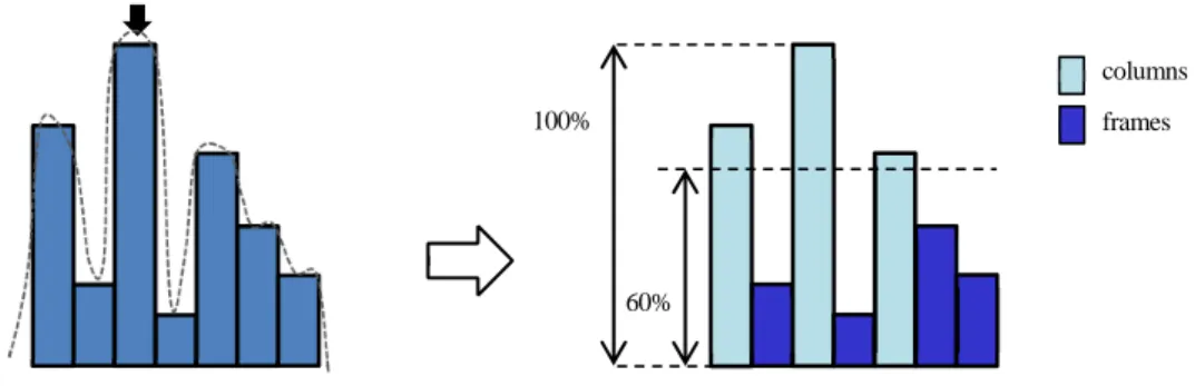
First, the highest rectangle is calculated from the partitioned 2D sketch. Then a threshold value, Th, is used to distinguish between columns (whose height is higher than the height of highest rectangle x Th) and frames (other rectangles), as shown in Fig. 6. Here, we set Th to 60%. A user can specify Th, from 30% to 60%, to change the characteristics of a processing plant.
Fig. 7 illustrates the procedure for generating a frame from a bounding box. A bounding box, which is labeled as a frame (red box in Fig. 7 (a)), is partitioned into lattices avoiding other boxes, as shown in Fig. 7 (b). Then, each floor is generated repeatedly, as shown in Fig. 7 (c). Here, the vertical, frontage and depth interval of each lattice can be changed with random numbers.
A bounding box which is labeled as a processing column is replaced with a column model in the following procedure.
(a) determining the extent rectangle of the site (b) column placement
Figure 5: Extent Rectangle of the Site and Column Placement
slide
Figure 6: Distinguishing between Columns and Frames
100%
60%
columns frames
(a) bounding box (b) partitioning (c) floor generation (d) result
3.4 Tank Arrangement
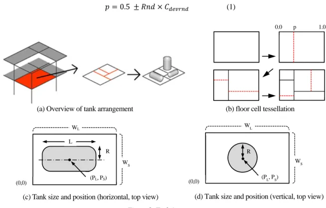
After frame generation, each floor is recursively tessellated into smaller rectangular cells until the size reaches a threshold value, and then each cell is filled with a tank, as shown in Fig. 8 (a). Fig. 8 (b) shows a result of the cell tessellation process. A tessellation position, p, gives a position in a normalized space (0.0-1.0), and is determined by Eq. (1). Here, Rnd is a uniform random number, and Cdevrnd is a parameter to control the
randomness of the tessellation position.
0.5 (1)
A tessellation direction, horizontal or vertical, is also controlled by the parameter, Cdevdir, which is in a range
from 0.0 to 1.0. The tessellation direction is fixed as horizontal when Cdevdir is set to 0.0 or as vertical when Cdevdir
is set to 1.0, or varied fifty-fifty when Cdevdir is set to 0.5.
After floor cell tessellation, a tank is placed into each cell by the following procedure.
(1) The algorithm determines stochastically whether to place a tank into a cell or not. A user can specify this probability to control density of tanks.
(2) Determine tank placement direction (lie down horizontally or stand vertically). This direction is also determined stochastically with a parameter to control the probability.
(3) Calculate the radius (R) and the length (L) of a tank. These sizes are calculated using the following equations, Eq.(2) and Eq.(3-1);
R _ _ _ (2)
L _ _ _ (3-1)
Here, Ws and WL are the lengths of major and minor axis, respectively. The range of radii is specified
by the parameters, Tmin_radius and Tmax_radius, and the range of length is specified by the parameters,
(a) Overview of tank arrangement (b) floor cell tessellation
Figure 8: Tank Arrangement
0.0 p 1.0 WL WS R L (PL, PS) (0,0)
(c) Tank size and position (horizontal, top view)
WL
WS R
(0,0)
(d) Tank size and position (vertical, top view)
Tmin_length and Tmax_length. Rnd is a uniform random number.
If tank placement direction is vertical, L is calculated from R, not from WL, as given by Eq. (3-2).
L R _ _ _ (3-2)
Here, Tmin_rate and Tmax_rate control the length of a tank. We set Tmin_rate = 3.0 and Tmax_rate = 10.0
respectively, after observing actual processing plants.
(4) The position of a tank, (PL, PS), is determined stochastically to be contained in a cell. There is also a parameter to control the randomness.
3.5 Piping
Finally, each outlet of a tank is connected to one selected adjoining lower tank by a pipeline, as shown in Fig. 9. The selection probability is inversely proportional to the distance between each outlet. A piping pattern is determined by the outlet directions and their relationships, as shown in Fig.10.
Ideally speaking, we should avoid collisions of a pipeline with other objects. However, it is a time consuming process to detect collisions, hence we omit this procedure in a practical way. Ikehira et al.presented an automatic design method for pipe arrangement using multi-objective genetic algorithms for optimizing the piping process. However, it took about 100 iterations to arrange 15 pipes. A processing plant contains over 100 pipelines usually, so a more effective method should be developed.
4.
Results
Fig. 11 illustrates the comparison of a real sample and a generated image. The black curve in Figure 11(b) is the sketch input specified by tracing a real sample, Figure 11(a). It is impossible to specify the precise depth data for each processing tower in our system, but we can observe similarity between the real sample and the generated image.
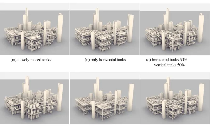
Fig. 12 shows the variations controlled by some parameters, such as the number of tessellations, the tank sizes, and the proportions of tanks, from the same input sketch data. Each image is rendered using skylight illuminance.
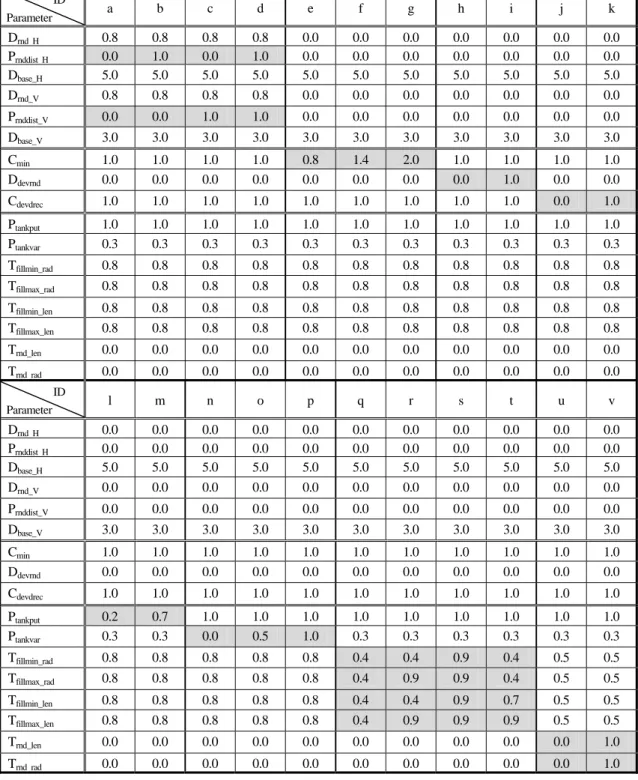
Fig. 13 shows the results generated by this method. Here, we show the effectiveness of parameter Th for generating frames, which is described in 3.3, in Fig. 13 (a-2) and (b-2). These two examples are obtained from the same sketch input, however we set Th to 30% for Fig.13 (a-1) and to 60% for Fig.13 (b-1), respectively. Therefore, we can change the appearance of the model drastically with parameter Th.
Opposite Orthogonal Same Facing
each other
Other
Figure 9: Piping Figure 10: Piping Patterns outlet
pipeline outlet
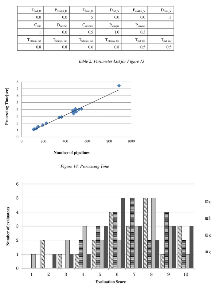
The processing time for generating tanks and piping depends linearly on the number of pipelines, as shown in Fig. 14. The time was measured on a PC with Intel Core2 Quad 2.83GHz, 4GB memory.
We conducted subjective evaluations for Figure 13. Each respondent evaluated the figures using a 10-point scale, with a higher number representing higher satisfaction. Figure 15 shows the evaluation results from 22 respondents. The average scores are 6.9, 7.3, 6.6 and 7.0, respectively. This result shows that the generated examples are highly evaluated.
5. Conclusion
The examples show that the landscapes of processing plants are satisfactorily represented, while some detailed parts, such as valves, steps, and branching pipelines, are not generated.
The method does not consider collisions of pipelines and other objects, either. Therefore, some pipelines penetrate tanks and processing columns. In general, a collision-detection process is a time-consuming one; therefore we have to design an effective way to avoid collision in the piping process.
From a practical application standpoint, it is necessary to edit a generated model interactively. For example, the operator will want to change the piping, tank layout, and tower placement. In our current implementation, we do not support interactive editing for a generated model. It is also necessary to texture massive models automatically, however this is outside our research scope.
We plan to address these issues in future research.
(a) real sample (b) traced 2D sketch input
(c) bounding box (d) generated model
Reference
Procedural Inc.(2008) CityEngine, http://www.procedural.com/
Frischer, B. et al.(2008) Rome Reborn, SIGGRAPH2008 New Tech Demos.
Parish, Y. I. H., and Müller, P. (2001) Procedural Modeling of Cities, Proc. of ACM SIGGRAPH 2001,pp.301-308.
Müller, P., Wonka, P., Haegler, S., Ulmer, A., and Van Gool., L.(2006), Procedural Modeling of Buildings, Proc. of ACM SIGGRAPH
2006/ACM TOG, 25, pp.614-623.
Müller, P., Zeng,G., Wonka, P., and Van Gool, L.(2007) Image-based Procedural Modeling of Facades, Proc. of ACM SIGGRAPH
2007, 26, #85
Chen, G., Esch, G., Wonka, P., Müller,, P., and Zhang, E. (2008) Interactive Procedural Street Modeling, Proc. of ACM SIGGRAPH 2008, 27, pp.1-10
Stiny, G. (1980) Introduction to Shape and Shape Grammars, Environment and Planning B: Planning and Design, 7, 3(May), pp.343-351.
Wonka, P., Wimmer, M., Sillion, F., and Ribarsky, W. (2003) Instant Architecture, ACM Transaction on Graphics, 22, 4 (July), pp.669-677.
Merrell, P., and Manocha, D.(2009) Constraint-based Model Synthesis, SPM '09: 2009 SIAM/ACM Joint Conf. on Geometric and
Physical Modeling, pp.101-111.
Merrell, P. (2007) Example-based Model Synthesis, I3D '07: Proc. of the 2007 Symposium on Interactive 3D Graphics and Games, pp.105-112.
Fujita, K., Akagi, S., and Doi, H. (1992) Automated Acquisition of Constraints in Plant Layout Design Problems, Journal of the
Japan Society of Mechanical Engineers, Vol.58, No.555, pp.3449-3454. (in Japanese)
Ohyama, K., and Ishii, T. (2007) Kojo Moe, Tokyo-Shoseki Co.Ltd (in Japanese)
Ikehira, R., Kimura, G., and Kajiwara H. (2005), Automatic Design for Pipe Arrangement using Multi-objective Genetic Algorithms,
(a) uniform frame distance (b) varied horizontal frame distance (c) varied vertical frame distance
(g) coarse cell tessellation (h) without cell tessellation (i) with cell tessellation deviation (minimum cell size = 2m) deviation
(j) tanks in same direction (k) tanks in random directions (l) few tanks
Figure 12: Variations
(d) varied horizontal and
(m) closely placed tanks (n) only horizontal tanks (o) horizontal tanks 50%
vertical tanks 50%
(p) only vertical tanks (q) all tanks are small (r) varied tank sizes
(v) randomly arranged tanks
Figure 12: Variations (continued)
ID Parameter a b c d e f g h i j k Drnd H 0.8 0.8 0.8 0.8 0.0 0.0 0.0 0.0 0.0 0.0 0.0 Prnddist H 0.0 1.0 0.0 1.0 0.0 0.0 0.0 0.0 0.0 0.0 0.0 Dbase_H 5.0 5.0 5.0 5.0 5.0 5.0 5.0 5.0 5.0 5.0 5.0 Drnd_V 0.8 0.8 0.8 0.8 0.0 0.0 0.0 0.0 0.0 0.0 0.0 Prnddist_V 0.0 0.0 1.0 1.0 0.0 0.0 0.0 0.0 0.0 0.0 0.0 Dbase_V 3.0 3.0 3.0 3.0 3.0 3.0 3.0 3.0 3.0 3.0 3.0 Cmin 1.0 1.0 1.0 1.0 0.8 1.4 2.0 1.0 1.0 1.0 1.0 Ddevrnd 0.0 0.0 0.0 0.0 0.0 0.0 0.0 0.0 1.0 0.0 0.0 Cdevdrec 1.0 1.0 1.0 1.0 1.0 1.0 1.0 1.0 1.0 0.0 1.0 Ptankput 1.0 1.0 1.0 1.0 1.0 1.0 1.0 1.0 1.0 1.0 1.0 Ptankvar 0.3 0.3 0.3 0.3 0.3 0.3 0.3 0.3 0.3 0.3 0.3 Tfillmin_rad 0.8 0.8 0.8 0.8 0.8 0.8 0.8 0.8 0.8 0.8 0.8 Tfillmax_rad 0.8 0.8 0.8 0.8 0.8 0.8 0.8 0.8 0.8 0.8 0.8 Tfillmin_len 0.8 0.8 0.8 0.8 0.8 0.8 0.8 0.8 0.8 0.8 0.8 Tfillmax_len 0.8 0.8 0.8 0.8 0.8 0.8 0.8 0.8 0.8 0.8 0.8 Trnd_len 0.0 0.0 0.0 0.0 0.0 0.0 0.0 0.0 0.0 0.0 0.0 Trnd rad 0.0 0.0 0.0 0.0 0.0 0.0 0.0 0.0 0.0 0.0 0.0 ID Parameter l m n o p q r s t u v Drnd H 0.0 0.0 0.0 0.0 0.0 0.0 0.0 0.0 0.0 0.0 0.0 Prnddist H 0.0 0.0 0.0 0.0 0.0 0.0 0.0 0.0 0.0 0.0 0.0 Dbase_H 5.0 5.0 5.0 5.0 5.0 5.0 5.0 5.0 5.0 5.0 5.0 Drnd_V 0.0 0.0 0.0 0.0 0.0 0.0 0.0 0.0 0.0 0.0 0.0 Prnddist_V 0.0 0.0 0.0 0.0 0.0 0.0 0.0 0.0 0.0 0.0 0.0 Dbase_V 3.0 3.0 3.0 3.0 3.0 3.0 3.0 3.0 3.0 3.0 3.0 Cmin 1.0 1.0 1.0 1.0 1.0 1.0 1.0 1.0 1.0 1.0 1.0 Ddevrnd 0.0 0.0 0.0 0.0 0.0 0.0 0.0 0.0 0.0 0.0 0.0 Cdevdrec 1.0 1.0 1.0 1.0 1.0 1.0 1.0 1.0 1.0 1.0 1.0 Ptankput 0.2 0.7 1.0 1.0 1.0 1.0 1.0 1.0 1.0 1.0 1.0 Ptankvar 0.3 0.3 0.0 0.5 1.0 0.3 0.3 0.3 0.3 0.3 0.3 Tfillmin_rad 0.8 0.8 0.8 0.8 0.8 0.4 0.4 0.9 0.4 0.5 0.5 Tfillmax_rad 0.8 0.8 0.8 0.8 0.8 0.4 0.9 0.9 0.4 0.5 0.5 Tfillmin_len 0.8 0.8 0.8 0.8 0.8 0.4 0.4 0.9 0.7 0.5 0.5 Tfillmax_len 0.8 0.8 0.8 0.8 0.8 0.4 0.9 0.9 0.9 0.5 0.5 Trnd_len 0.0 0.0 0.0 0.0 0.0 0.0 0.0 0.0 0.0 0.0 1.0 Trnd rad 0.0 0.0 0.0 0.0 0.0 0.0 0.0 0.0 0.0 0.0 1.0
(d-1) sketch #4 (d-2) example#4
Figure13: Examples
(c-1) sketch #3 (c-2) example #3
(a-2) example#1 (b-2) example #2
Drnd_H Prnddist_H Dbase_H Drnd_V Prnddist_V Dbase_V
0.0 0.0 5 0.0 0.0 3
Cmin Ddevrnd Cdevdrec Ptankput Ptankvar
1 0.0 0.5 1.0 0.3
Tfillmin_rad Tfillmax_rad Tfillmax_rad Tfillmax_len Trnd_len Trnd_rad
0.8 0.8 0.6 0.8 0.5 0.5
Table 2: Parameter List for Figure 13
Figure 14: Processing Time
Figure 15: Subjective Evaluations for Figure 13
0 1 2 3 4 5 6 7 8 0 200 400 600 800 1000 Proces si n g Time[s ec] Number of pipelines 0 1 2 3 4 5 6 1 2 3 4 5 6 7 8 9 10 a b c d Evaluation Score Nu mb er of evalu a tors