ウェブスターのホーン方程式における摂動論による高精度計算手法

(1)

ウェブスターのホーン方程式における摂動論による高精度計算手法

濱野慶太1,坂本昇一2,富谷光良*3

Highly Accurate Perturbative Method for Webster's Horn Equation

Keita HAMANO * 1, Shoichi SAKAMOTO * 2 Mitsuyoshi TOMIYA * 3

ABSTRACT : Applying mathematical and quantum mechanical techniques, this study develops numerical

solutions to Webster's horn equation, which describes the sound inside brass instruments in acoustics. The

wavenumbers and wave functions of the modes in the system are evaluated by perturbation theory, assuming

a solvable system with relatively small perturbations. An obvious solvable example is a straight pipe, whose

wavenumbers can be perturbed by varying the radius of the horn. Maintaining the second-order corrections,

the method generated astonishingly accurate results for varying horn shapes. Moreover, in tests of various

pipe shapes, the perturbation method required far fewer computational resources than the finite element

method. Two analytically solvable shapes and two non-solvable models (one of them is a periodic shape

described by a trigonometric function) are analyzed. The results imply the applicability of the method to

highly non-solvable systems.

Keywords : Webster's Horn Equation, Perturbation Theory, Brass Instruments, High Accuracy Solutions

(Received June 8, 2018)

1 INTRODUCTION

Lately, sophisticated tools designed for solving nonlinear problems have been successfully applied to studies of wind instruments. In particular, these tools can analyze the resonance phenomena and predict the sound propagation and reflection inside finite spaces such as pipes)) A typical application reveals the dynamic function of the register hole on the clarinet, which comprises a two-delay system.2)

However, the sound making methods and resonance mechanisms of musical instruments have not been sufficiently unravelled.1) 3) Even simply structured instruments such as recorders remain incompletely understood. Therefore, investigating these mechanisms is essential for the research and development of wind instruments. One promising approach toward a precise and manageable design method for specific

*1:理工学研究科物質生命理工学専攻修士学生 *2:物質生命理工学専攻助教

*3:物質生命理工学専攻教授(tomiya@st _{.seikei.ac.jp)}

instruments is the technique in quantum mechanics, which naturally describes wave dynamics. The expected close relationship between acoustics and quantum mechanics should exactly fulfil our intention.4>

As a representative brass instrument, a trumpet can be divided into three parts: a lead pipe, a piston unit and a horn (also called a bell).1)'3) The lead pipe amplifies the sound, the pistons control the pitch and the horn acts as a speaker. Additionally, the horn is easily manufactured in various sizes and shapes, and from a variety of materials. Indeed, the horn is merely the aperture of the instrument, and its tone is easily supplemented by distinguishing characteristics.

The normal modes and frequencies of the horn can be altered by adjusting the horn structure. Understanding the relationship between the modes and structure of a horn is crucial in instrument manufacture. The pressure changes inside the horn are well approximated by Webster's horn equation,5)'6) which is generally solved by numerical methods; analytical solutions can be obtained only in some special cases. However, the balance of the musical instrument can be disrupted by

(2)

numerical errors, which are unavoidable

in numerical analyses.

In this work, we approach the acoustics in a horn from a

quantum mechanics perspective. The perturbation method,

which derives the solutions of Schrodinger

equation with small

perturbations,7) can evaluate the modes of brass

instruments.8>'9)

For various horn shapes, the approximate

solutions computed by perturbation theory are far more

accurate than those of ordinary numerical methods such as the

finite element method (FEM)Iom

0 and the eigenfunction

expansion method.6'12)'13)

Although quantum physics underlies the modern science of

the twentieth century, the perturbation method was originally

developed

to explain the motions of planets in the solar system,

and stars in galaxies, and similar problems in classical

astrophysics.14>

The Webster's equation, which describes

the sound in a pipe

with varying radius,10>

can be mathematically likened to a

perturbed Schrodinger equation.8)'9)

Thus, perturbation theory

can be applied to the acoustics of brass instruments.

Perturbation

theory divides the system into a non-perturbative

and a perturbative

part. The former part usually admits an exact

solution, whereas the latter is expressed

as an asymptotic series

expansion with respect to the perturbation term, assuming a

sufficiently

small perturbation

strength. This formulation

gives

an approximate solution to systems with no exact analytical

solutions.

Our system treats the horn structure as a straight pipe

(exactly solvable) with some deformations (perturbations),

which model the deformation of the stationary states. The

method returns precise results for the rotation volumes (one

revolution around the x-axis) of four horn structures,

proportional to e x , 1/x, 3+ cos x , and ln(x) (x>0). Ordinary

numerical methods such as FEM usually perform best in the

lower frequency region, because the lattice constant must be

smaller than the wavelength. In contrast, the perturbative

method usually achieves better results in the higher frequency

region than FEM.

2 WEBSTER'S EQUATION AND SCHRODINGER

EQUATION

Sound is the physical phenomenon manifesting from the propagation of pressure changes through a medium such as air. If the wavelength is sufficiently larger than the horn diameter, the propagation becomes essentially one-dimensional and is

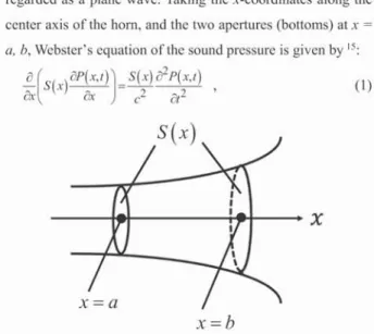
regarded as a plane wave. Taking the x-coordinates along the center axis of the horn, and the two apertures (bottoms) at x = a, b, Webster's equation of the sound pressure is given by 15:

a's(x)aP(,r)`s(~

~

)a~(~,t)

(1)

ax,

S(x) .

1

x x=a i. x=b

FIG. 1. Outline of the pipe to be used in Webster's equation

where P(x,t) is taken here as the acoustic or excess pressure, which is the pressure difference from the static one, S(x) represents the varying cross-sectional area of the horn part (FIG.1), c is the speed of sound, and t is time.

The Schrodinger equation for an exactly solvable system with Hamiltonian H0 is given by

H0VI0

,n = E0,nyI0,n ,(2)

where Vnis an eigenstate of the solvable system with eigen-energy E0,n• The Schrodinger equation with a small perturbation H1 then becomes

Hyin

= (H0 + H1) vin = Eyi .

(3)

The term H1 can be any suitable term, such as a potential energy, an interaction term or a perturbative part.

Quantum mechanics is a powerful tool for handling systems that satisfy the perturbation equation (3). Perturbation theory derives the energy spectra and wavefunctions of perturbative systems from those of the solvable system, adding correction terms generated by expanding the perturbation. Traditional quantum mechanics7 gives the second-order energy correction as

2

(1VO,kVil1VO,n)((4)

En

=EOn+(VO

_{,nVHlVO,n)—~4}

knEO,n –EO,k and the first-order correction of the wave function as

Yin= iVOn+1VO,k

1(1VO,kVii

i'O,n)

.(5)

knEO,n —EO,k

(3)

Later, we will apply the one-dimensional Schrodinger equation

with a potential V (x)

2 – h a 2+ V (x)Yin = Enyin ,(6) 2m ax

where h is the Planck constant and m is the mass of the particle that follows Eq. (6). Comparing Eqs. (3) and (6), we find the general relations

h2 a2 H

o=---H1=V, H=H0+V.(7) 2

m ax2

Therefore, we expand the perturbation with respect to V.

3 PERTURBATION THEORY FOR WEBSTER'S

EQUATION8'9

To clarify the resemblance between the Webster's and Schrodinger equations, we try a change of variables in Webster's equation (1) as follows:

'Fn (x,t) = Pn (x,t) jS(x)(8)

r (x) = vIS

(x) ,(9)

where r is clearly proportional to the radius of its cross-section at x. The time dependence of P is separated by the factor eiwt

Pn (x ,t) = Pn (x)eiwt(10)

Here 0) is the angular frequency and

k = (11)

is the wavenumber of the wave. The equation (1) then transforms into

–d2 yin

2+r„y'_kn2yin(12) dxr

where

the

eigen-

"wavefunction":

_{iin (x) is also introduced}

_as

gin (x,t) _ vin

(x)eiwt(13)

Putting E_{n=k,72 and h = 2m =1 , we obtain Schrodinger} equation for one dimensional scattering (6), where k2

n expresses the energy of the particle and the potential energy

V (x) becomes r"/r . Note that n labels the

eigen-wavenumber k_{n and the eigen-energy} _{En in a finite region,} i.e., within the space of the brass instrument. The Hamiltonian of the system becomes

d2 r„ H =H0+V=–

2+—(14) dxr

Thus, the potential

energy term r"/r plays a perturbative

role.

Different from Schrodinger equation, we do not normalize

yin

(x) , because

the

term yin

(x)IIS(x) represents

the

sound

pressure at x. Therefore, the normalization would remove some important information.

Perturbation theory is applicable when the contribution of the perturbation H1 = V = r is relatively small. To obtain the difference between k0,n2 of the straight pipe and kn2 with a second-order perturbation V, we modify Eqs. (4) and (5)

as 2 Y

~)_~1---

z 21Y" —1 , (15) k n = k0+YnYiO,nYY~O,nrk22Yn mnk0,n— k0,m r" Y1O,m rY1O,n16 Y/n =1110,n +2 2 7nYO,n() mn kO,n -kO,m

where the symbols in (15) and (16) are respectively defined as r"b r"

(1ff

0,n ,m)

' VO,n

—vto,mdx(17)

a and b

Yn=~1VO,n2dx•(18)

a The factor yn is introduced for acoustical applications. In

quantum mechanics, the wavefunctions yin must be

normalized

as yn =1 , because yin (x)2 dx represents

the

probability that a corresponding particle exists in the range

[x, x+dx] . Therefore,

integrating

all probabilities

of a particle

existing in that region, we obtain

Jb

a2(l ,(19)

implying that the particle is somewhere inside the whole range

[a, b] .

As a non-perturbative system, we solve Webster's equation in a straight pipe. The non-perturbative system should be solvable and admit a series of analytical and exact solutions

vn(x)

A straight-pipe

system is obtained

by neglecting

the potential

energy term r"/r . The solution of the non-perturbed

Eq. (12)

is

1VO

_,n

_(x)

_{= An}

_cos

_(kpnx)

₊

_Bn

_sin

_(kpnx)

_.

₍₂₀₎

The boundary condition quantizes the wavenumber k. The general solution for the straight pipe, obtained by summing the

kn , is the following Fourier decomposition, as expected:

(4)

1'o(x)=L1'O

_,n(x)

n(21)

= L{An

cos(ko

nx)+Bn

sin(ko

_,nx)}

n As the horn is open-ended at both sides, u must be 0 at both ends x = a and x = b . Thus, the boundary conditions are

tan

_{(ko,na) = tan (ko,nb)}

_{= - An}

_1B

_;

_{equivalently,}

sin

{k

(b - a)}

= 0 . Thus,

the

wavenumbers

are

quantized

as

n7cnic() k 0'n22 _{b -a} _L

Under this boundary condition, Eq. (21) becomes

11/o

=I Bn

{sin

(ko

nx)-tan(ko

n)cos(ko

nx)} (23)

n

Eq.

(22)

also

offers

the

eigen-frequency

fo,n = cko n /271"

= en/2(b - a) of the sound wave in the straight

pipe. (al Solvable system R I , 0 a

L

~ x

Strai2ht (h) R Perturbative

j{r(x)

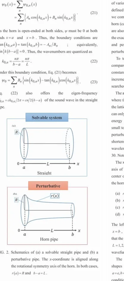
I I I /I I VI 0 J a L '.x b Horn pipe

FIG. 2. Schematics of (a) a solvable straight pipe and (b) a perturbative pipe. The x-coordinate is aligned along

the rotational symmetry axis of the horn. In both cases,

r(a)=Rand b-a=L.

4 NUMERICAL CALCULATION MODELS

The shape of a horn pipe can be modeled by various functions. In this paper, we apply perturbation theory to horns

of various shapes. Each shape is determined by rotating a body defined by the function r(x) around the x-axis. For each shape, we compare the solutions of the straight pipe and the varying horn (calculated by perturbation theory)(FIG.2). The solutions are also compared with those of typical numerical methods. If the exact solution is obtainable, comparisons between the exact and perturbative solutions will validate or invalidate the perturbation method.

To test the accuracy and efficiency of our method, we compare our results with those of FEM10,11. The lattice constant is set to AK = 0.001 . The energy E = k2 is incremented by AE = A(k2) = 0.0002 , and the eigenstates are searched.

The accuracy of FEM usually deteriorates at higher energies, where the wavelength becomes comparable to or smaller than the lattice constant Ax . Therefore, computational approaches can only roughly approximate the physical phenomena in high-energy regions. The lattice constant must be set sufficiently small to prevent this degradation. The wavelength of the

non-perturbative system A0,

n= 27z/ko,12

= 2L/n

reduces as L

shortens and/or n increases. In our work, the shortest

wavelength

_{is 4 ,30 = 2 x 1/30 = 0.06667...}

_{» Ox for L= 1 and n =}

30. Note that 20,30 is more than sixty times larger than Ax .

The x-coordinate

of Webster's equation must align along the

axis of rotational symmetry of the pipe (namely, through the

center of the pipe). In the perturbative systems, the shapes of

the horn pipe are given by the following functions

(see FIG. 3):

(a) r (x) = e-x

(b) r (x) =1/x(24)

(c) r(x)=3+cosx

(d) r(x)=lnx

.

The left and right ends of the pipe are located at x = a and x = b , respectively. The pipe length is L=b-a . To ensure that the pipe shape changes gradually along its length, we select L = 1, 2,... ,10 , and determine the wavenumbers k and wavefunctions'n for n= 1, 2,... , 30 .

The end positions are set to a= 0, b= L for potential shapes (a) and (c), a= 1, b = L + 1 for shape (b) and a = e, b = e+L for shape (d). When a=0 , the boundary conditions reduce to the simple forms An = 0 and

tan

(k120

b) = 0 , and

the

result

becomes

Eq.

(22).

This section focuses on V n rather thanPn = vn l j ,

because the effect of varying the radius is much easier to distinguish in ln than in pressure. Different from their usual

(5)

definitions, both "energy" and "potential" have units of m-2 and are so named only by mathematical analogy between the Webster's and the Schrodinger equations.

r (x)

=L

„'

0b

r (x) = e-x (a)

'.L0 Ib

r(x)=

r

r(x)=3+cosx

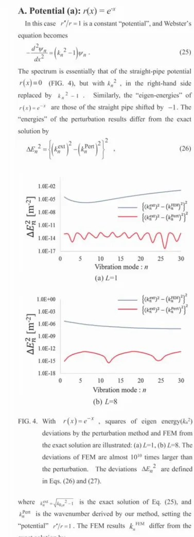
A. Potential (a): r(x) = ex

In this case r"/r =1 is a constant

"potential",

and Webster's

equation

becomes

d2d'n(k

_n2

_{_ l)vn.(25)}

dx2

The spectrum is essentially that of the straight-pipe potential

r(x) = 0 (FIG. 4), but with kn2 , in the right-hand

side

replaced by k 2 - 1 . Similarly, the "eigen-energies" of r (x) = e-x are those of the straight pipe shifted by -1. The "energies" of the perturbation results differ from the exact

solution by 2

AEn2

= (knxt)2(kPert)2(26)

r(x)

I. L_,..1

elb

x

r(x)=1nx

Schematics of the pipe shapes investigated in

perturbation

study: (a) r(x) = e-x , (b) r(x) =1/x ,

r(x)=3+ cos

x, (d)r(x)=1nx.

the (c) 1.0E-02 r^1.0E-052

b{(knxt)2

_ (k~`EM)2)

`J 1.0E-08j(knxt)2

_{_(knert)212}

.~ 1.0E-11I)

<I 1.0E-17 0 5 10 15 20 25 30 Vibration mode : n (a) L=1

1.0E+00---

{(knxt)2

_ (knEM)212

1.0E-03{(knxt)2

_ (knert)2)2

N

IE 1

_.0E-06

CV1.0E-09

41.0E-12

1.0E-15

1.0E-18

0

5

10

15

20

25

30 Vibration

mode : n

(b) L=8

FIG. 4. With r (x) = e

, squares of eigen energy(kn2)

deviations

by the perturbation

method

and FEM from

the exact

solution

are illustrated:

(a) L=1, (b) L=8. The

deviations

of FEM are almost 101°

times larger than

the perturbation. The deviations

AEn2 are defined

in Eqs. (26) and (27).

where knXt

= jkOn2

_ 1 is the exact solution

of Eq. (25), and

kPert

is the wavenumber

derived

by our method,

setting

the

"potential" r"/r =1 . The FEM results k

_nFEM

_{differ from the}

exact solution

by

FIG.3.

(6)

AEn2_(knxt

)2

—(kkEM)22(27)

where kn

EM is the wavenumber

obtained by FEM.

The calculation which can be estimated in this case, because the exact solution is obtainable. The deviation result AEn2 of the perturbation method is strikingly superior (by 10 orders of magnitude) to the FEM result. The deviations from the exact squared "energies" approach the precision limit of the computational program (FIG. 4). Of course, the wavefunctions are identical to those in a straight pipe.

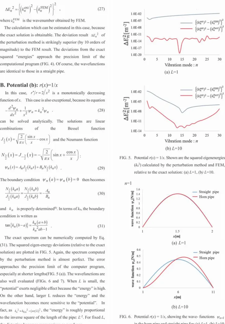
B. Potential (b): r(x)=1/x

In this case, r"/r= 2/x2 is a monotonically

decreasing

function ofx. This case is also exceptional, because its equation

_d22n

_{+ 2 yin = kn2~n}

_.

(28)

dxx

can be solved analytically. The solutions are linear

combinations of the Bessel function

2 ~sinx

J3 (x) _—cos

x and the Neumann

function

2Tcxx

/

N3 (x)=J _3 (x)=—?sin

x+cosx

2271"x \x •

n (x) = AnJ3

22

(knx)+BnN1

(knx) .(29)

The boundary

condition yin (a) = yrn (b) = 0 then becomes

Nz(kna)N3(knb)

A

n

J

2(kna)J2(knb)B(30)

and k is properly determined8). In terms of kn, the boundary condition is written as

tan{kn

(b—a)}

=kn

(a+b)

2(31) k nab—1

The exact spectrum can be numerically computed by Eq. (31). The squared eigen-energy deviations (relative to the exact solution) are plotted in FIG. 5. Again, the spectrum computed by the perturbation method is almost perfect. The error approaches the precision limit of the computer program, especially at shorter lengths(FIG. 5 (a)). The wavefunctions are also well evaluated (FIGs. 6 and 7). When L is small, the "potential" exerts negligible effect because the "energy" is high. On the other hand, larger L reduces the "energy" and the wavefunction becomes more sensitive to the "potential". In fact, as kn2 ,k00,2=(nr/L)2,the "energy" is roughly proportional to the inverse square of the length of the pipe: L-2. For fixed L, the distortion becomes more serious as n reduces.

u N g W 1.0E-02 1.0E-05 1.0E-08 1.0E-11 1.0E-14 1.0E-17 1.0E-20 1.0E-02 1.0E-05 N g 1.0E-08 W <I 1.0E-11 1.0E-14 0 0 ll(kRxt)2 —(llknEM)21z --- j(knxt)2_(knert)2J12 5 10 15 Vibration mode (a) L=1 20 :n 25 30

(04xt)2

—

(k

{(knext)2_(k

)2}2

FIG. 5. Potential r(x) = 1/x. Shown are the squared eigenenergies (k„2) calculat relative to the n=1 1.6 1.4— Straight pipe 1.2— Horn pipe ~'1 O 0.8

co0.6

w

_0.4

ct0.2

0

11.52 x[m]

(a) L=1

0.6 — Straight pipe

Z0.5—

Horn

pipe

b. 0.4

O 0.3

•

0.2 >0.1

0 1611

x[m]

(b) L=10

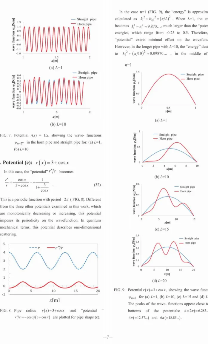
FIG. 6. Potentialr(x) = 1/x, showing the wave- functionsy'n=1

in the horn pipe and straight

pipe for: (a) L=1, (b) L=10.

5

10

15

20

25

30 Vibration mode : n

(b) L=10

1/x. Shown are the squared

eigenenergies

f xl by the perturbation method and FEM,

(7)

--- ~1 .9 1.4 •0.9 0 * -= 0.4 -0.1 cD -0.6 -1.1 -1.6 — Straight pipe — Horn pipe

11.52 x[m]

(a) L=1

— Straight pipe

o.s—Horn

pipe

• •

z0.4,

• Y 0 , ft 4 $$•

0.3 0.2 O 0.1 4 ,,0• 4, -0 .1

w -0.2

C'-0.50O~OO~~O•

0.4 ,0

• 3 -0.6

1611

x[m]

(b) L=10

FIG. 7. Potential r(x) = 1/x, showing the wave- functions

yrn_27

in the horn pipe and straight

pipe for: (a) L=1,

(b) L=10

. Potential

(c): r (x) = 3 + cos x

In this case, the "potential"

r"/r becomes

rn COSx 1

r3 + cos x1 + 3(32)

cos x

This is a periodic function with period 27r (FIG. 8). Different from the three other potentials examined in this work, which are monotonically decreasing or increasing, this potential imposes its periodicity on the wavefunction. In quantum mechanical terms, this potential describes one-dimensional

scattering. 5 4 • 3 2 1 0 0 -1 ---r _Y"/r FIG. 8. 0

xi ml

Pipe radius

r (x) = 3 + cos x

and "potential

r"/r = —

cos x/(3 + cos x) are plotted for pipe shape (c).

In the case n=1 (FIG. 9), the "energy" is approximately

calculated

as k12 k0,12

=(ir/L)2 . When L=1, the energy

becomes kt2 =R-2, 9.870..., much larger than the "potential" energies, which range from -0.25 to 0.5. Therefore, the "potential" exerts minimal effect on the wavefunction

. However, in the longer pipe with L=10, the "energy" deceases

to k12 (410)2 0.09870... , in the middle of the

n=1 1.5 _{— Straight pipe} — Hom pipe

a 0.5

V 7 0.51 x[mJ (a) L=1 — Straight pipe — Horn pipe

10:

0

_Aar

2 4 6 8 10 x[mI (b) L=10 0.6 £— Straight pipe - Horn pipe g.0.4 V I 0.2 0 0510 15 x[mI (c) L=15 0.5 — Straight pipe z 0.4-Hom pipe

cg

0.2 frv'

i, 0.1

0

510

15

20 x[mI

(d) L=20

FIG. 9. Potential r (x) = 3+ cos x , showing the wave functions

Vn=1 for (a) L=1, (b) L=10, (c) L=15 and (d) L=20.

The peaks of the wave- functions appear close to the

bottoms of the potentials: x = 27-c(=

6.283...) ,

47r(=12.57...)

and 67r(=18.85...)

.

(8)

-7-"potential" energy range (32). Consequently,

the wavefunction

is enhanced near the bottom of the "potential" r"/r , and

diminished around the peaks. In quantum mechanical terms,

the wavefunction

defines the probability that a particle will be

found at a specific point in the system. The peaks indicate

regions of low probability of finding a particle. Particles are

most likely to exist in the bottoms of the "potentials".

In FIG. 9, the waves in longer horns exhibit multiple peaks

imposed by the periodic "potential". All wavenumbers are

n =1 , denoting ground states or first modes. The pressure

P(x,t) can be enumerated from the wavefunction

(x ,t)

by Eq. (8). The pressures exhibit a single peak (FIG. 10), which

typifies the first mode in a finite region.

0.20.6

E

E 0.1

ytA 0 FIG. 10. FIG. -Pressure wave function 0.5 0.4 0.3 0.2 0.1

\ 0

0510

15 x]m]

Pressure P(x) and wavefunction

>/rn

(x)

potential r"/r = —

cos

x/(3 + cos

x) with n

L=15.

The pressure

has just a single

peak, all

is quite distorted.

n=27

_-Straight

pipe

-Hom

pipe

E1.5 . .

.

. .

l

c 0.5

0 u 0 a -0.5 Rd >-1 -1.5 E 0.5 y 0 + -0.5 E z 0 U

x) in the

n=1 and

although

it

0 0.5 x[m] (a) L=1

-Straight pipe -Horn pipe

0510

x(m]

(b) L=10

11. Potential r (x) = 3 + cos x , showing the wavefunctions

Y

n=27 for: (a) L = 1 and (b) L = 10. In case (b), the

wavefunction

is slightly affected by the "potential".

In the higher mode n=27 (FIG. 11), k272

r-z,k0272

=(27ir/L)2

exceeds the "potential". For example, if L=1, then

k272 k0,272

=(272r)2

7200 , outrageously larger than the

"potential" . In this case, the wavefunction is barely influenced by the "potential" (FIG. 11). Even in the longest horn examined in our work (L=10), k272 72 is considerably larger than the "potential" . To observe this apparently unusual wave distortion, we require an unrealistically long horn (e.g., L=100).

D. Potential (d): r(x) = ln(x)

The "potential"

r"/r = —1/(x21n

x) becomes

very small

and negative

in the range

[e, e+L] (r"/r = —0.1353...

at

x = e ), and gradually

approaches

the x-axis.

Initially,

we

simply

multiply

the representative

potential

(a) by —1/1n

x •

Of course, the shape changes drastically toward small x, but this region is discarded. In the valid range, this potential varies much more slowly than the other potentials. As already explained, the energy is also much higher than the potential, so the wavefunction resembles that of the straight pipe over the whole parameter range tested in this study (FIGs. 12 and 13). Nevertheless, the wavefunction slightly distorts in longer systems. n=1 1s _-Straight_pipe -Horn pipe u

a0.5

0 2.63.13.6 xIm] (a) L=1 FIG. z 0.5 0.25 0 2.6 — Straight pipe — Horn pipe 12. Potential 'Vn=1 for _{_} exerts negligible effect in both length cases.

7.2

11.8 xImJ

(b) L=10

functions

potential"

—8—

(9)

n=27 E 1.5 z

~ 1

G 0.5 0 e 0 '-, •-0 .5 eta -1 -1 .5 E 0.5 z 0 a ^0 ca 2.6

3.13.6 x[m]

(a) L=1

_-0.5

2.65.2

7.8

10.4 x[ml

(b) L=10

FIG. 13. With r (x) =1n x , graphs of wave function Vn_27

are illustrated in the cases : (a) L=1, (b) L=10. The

effect of the "potential" is really limited.

5 SUNNARY AND DISCUSSIONS

This paper applies perturbation theory to Webster's equation (1), and derives second-order perturbation expression for horns of various shapes. Successful application of the theory to Webster's equation was confirmed in comparisons with the exact solutions. The wave number kr, and the sound pressure

Pn = p',z

/ J

were correctly enumerated.

Moreover,

this

method was applicable to pipes that markedly deviated from the straight pipe (the simplest solvable shape). Moreover, this method was viable for variously shaped brass instruments.

The calculation can be performed at much higher precision, and with remarkably less numerical computation, than FEM. On a paralleled workstation of several CPUs constructed in our laboratory, the FEM required 20-30 minutes' runtime for each given set of L and n. On the other hand, our method enumerates the cross integrations (16) almost instantaneously.

The longer the instrument, the larger the effect of the perturbation, because the wavefunction in the horn becomes more distorted. However, the perturbation method is much

more resilient to shapes that deviate from straight pipes than initially expected.

We believe that the exponential horn is the preferred design for brass instruments, because of its nearly flat frequency characteristics 1. However, real musical instruments have more delicate structures, for reasons that are not fully understood. When played, the instruments must deliver high-quality sound that changes continuously. Therefore, their dynamical properties must be studied. In subsequent investigations, we will investigate the time dependent characteristics of the horn shapes in a theoretical framework.

The time-dependent acoustical wave equation differs from the quantum Schrodinger equation. The former involves a quadratic time differential, whereas the latter has a first-order time differential. This mathematical difference complicates the analysis, and likely requires a new mathematical approach.4),16)

References and 1. 2. 3. 4. 5. 6. 7. 8. Links

Eric J. Heller. Why You Hear What You Hear: An Experiential Approach to Sound, Music, and Psychoacoustics. Princeton University Press, Princeton, (2012).

Kin'ya Takahashi, Kana Goya, and Saya Goya, "Mode Selection Rules for Two-Delay Systems: Dynamical Explanation for the Function of the Register Hole on the Clarinet", J. Phys. Soc. Jpn. 83, 124003 (2014).

Arthur H. Benade, Fundamentals of Musical Acoustics, Dover Publications, 391-411 (1990).

Mitsuyoshi Tomiya, Yosuke Sasaki and Shoichi Sakamoto, "Numerical Analysis of Dynamical Scar in Sound

Propagation", Proceedings of the 12th Western Pacific Acoustics Conference 2015, P9000179,

http://wespac2015singapore.com/eproceedings/html/P90 00179.xml (2015).

David T. Blackstock, Fundamentals of Physical Acoustics, A Wiley-Interscience publication, 251-254 (2000). P. A. Martin, "On Webster's Horn Equation and Some Generalizations", J. Acoust. Soc. Am. 116, 1381-1388, (2004).

Walter Greiner, Quantum Mechanics: An Introduction 4th Edition, Springer-Verlag, Berlin, Heidelberg, New York, 273-277(2001).

R. Jorge, arXiv: 1311.4238v1, physics.flu-dyn., (2013).

(10)

9. 10. 11. 12. 13. 14. 15. 16.

A.H.Benade and E. V. Jansson, "On Plane and Spherical Waves in Horns with Nonuniform I. Flare, "Theory of

Radiation, Resonance Frequencies, and Mode

Conversion", Acustica 31(2), 79-98, (1974).

Ichiro Kawakami, Masamitsu Aizawa, Katsumi Harada and Hiroyuki Saito, "Finite Element Method for Nonlinear Wave Propagation", J. Phys. Soc. Jpn. 54,

544-554 (1985).

Antoine Lefebvre and Gary P. Scavone, "Characterization of Woodwind Instrument Toneholes with The Finite Element Method", J. Acoust. Soc. Am. 131(4), 3153-3163

(2012).

Roger Waxler, "A Vertical Eigenfunction Expansion for The Propagation of Sound in A Downward-refracting Atmosphere", J. Acoust. Soc. Am. 112(8), 2541-2552

(2002).

Yusuke Naka, Assad A. Oberai and Barbara G. Shinn-Cunningham, "Acoustic Eigenvalues of Rectangular Rooms with Arbitrary Wall Impedances Using The Interval Newton/generalized Bisection Method", J. Acoust. Soc. Am. 118(6), 3662-3671 (2005).

Roger R. Bate, Fundamentals of Astrophysics, Dover Publications, 385-427 (1971).

A. G. Webster, "Acoustical Impedance, and The Theory of Horns and of The Phonograph," Proc. Natl. Acad. Sci. U.S.A. 5, 275-282 (1919).

Keita Hamano, Shoichi Sakamoto and Mitsuyoshi Tomiya, "High Accuracy Solution and Shape Universality of

Webster's Equation in High Frequency Region by Perturbation Theory", Proceedings of the 12th Western Pacific Acoustics Conference 2015, P9000185, http://wespac2015singapore.com/eproceedings/htm 1/ P9000185.xml (2015).

ウェブスターのホーン方程式における摂動論による高精度計算手法