On the linear equations calculating the shallow groundwater temperature near the water table from the air temperature in the paddy fields-香川大学学術情報リポジトリ

(1)

Vol 20, No 1 (1968) 75

ON THE LINEAR EQUATIONS CALCULATING THE SHALLOW GROUNDWATER

TEMPERATURE NEAR THE WATER TABLE FROM THE AIR TEMPERATURE

IN THE PADDY FIELDS

Kiyoshi

FUKUDA

Katsuhiko

I z u ~ s u

and Tadao

MAEKAWA

1. Introduction

Because the temperature of water and soil directly effects the growth of crops, it is important to know the temperature of water, including shallow groundwater, as well as to know their quantity.

Therefore a lot of investigations have been undertaken by many concerning this problem. Some have trid to construct an equation to calculate the values of soil temperature. For example, AZUMA ( 5 ) con-

structed a linear equation to calculate the yearly average temperature of soil from the yearly average air temperature.

What we have tried here, however, is to construct a linear equation by calculating the values of shallow groundwater temperature (S.G.T) near the water table from air temperature for a given area for a given month.

The paper presented here shows the results of our efforts. This is the 12th report of "The shallow groundwater in the downstream basin of the Aya River, Kagawa Prefecture".

2. Theory

When we plotted the values of the shallow groundwater temperature (S.G.T.) near the water table or

eg

(OC) (y-axis) against the observed values of the air temperature (A.T,) or Oa (Oc) (x-axis) at the area where the values of S.G.T. were observed, we obtained the closed lines showing the Og - Ba relationship as shown in Fig. 1.

These closed lines told us that we could not use the straight lines (the linear equations) to show the

Og

-

Oa relationship if we wanted to construct an equation to show this relationship.

However, if we could find the linear relationship between Og and Oa shown in Fig. 1, we could construct a linear equation (simple and most practical) to show the Bg

-

Oa relationship.

Therefore, to obtain the linear equations, we divided a year (12 months) (Fig.1) into three periods I, I1 and 111.

They were:

Period I = four months-January to April; Pe~iod I1 = three months-May to July; and Period I11 = five months-August to December.

(2)

Tech.. Bull. Fac. Agr. Kagawa Univ.

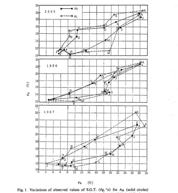
Fig. 1 Variations of observed values of S.G.T. (Bg, OC) for AR (solid circles)

and for Ar, (open circles) during 1965 (top figure), 1966 (middle figure) and 1967 (bottom figure). J represents January, F, February and so on

Through this method, the relationship between Og and t'a during each period seemed to be roughly a linear relationship as shown by the straight lines in Figs.3, 4, 5 and 6.

Therefore, for period I, we constructed Eq. (1) to show the 0,

-

t'a relationship

egI

= loa I

+

b

...

(1)

For period 11, we constructed Eq..(2),

...

t ' g ~ = mealI

+

c (2)

For period 111, we also constructed Eq.(3),

(3)

Vol. 20, No. 1 (1968)

where

Bg I

,

Ogl[ and Bgm = The values of S.G.T or 8, for the periods I, I1 and I11 respectively, (Oc).

B a l

,

Ban and Bam = The air temperature for the periods I, I1 and I11 respectively, (OC).

I, rn and n = The coefficients of 0 a for the periods I, I1 and I11 respectively. b, c and d = The constants for the periods I, I1 and I11 respectively.

To calculate the values of I, m and n, and b, c and a', we used the method of least squares (8) and con-

structed Eqs.(4), (5) and (6).

B g r B a r -0g11 @ a ~

- -

_...

m=

-

,

c = B g r - m B a r (Ban: 2,

-

( B a n (5) B g n B a n -8gm Barn

--

-

_...

a =

-

d=Ogmr

-

noann (Barn ' ) -

(G)

'

(6) 3. Data

The values of 0, were the arithmetic mean of the field data obtained from 51 observation wells (crosses in Fig.2). We referred to these values as the average values of Bg of the regions AR and AL on the day that observations were made. The field data was obtained from the shallow groundwater investigations that we have been carrying out ever since July 1964 by using 51 wells in the downstream basin of the Aya River, Kagawa Prefecture ( 1 7 2, 3 > 4> 6) (Fig.2).

Fig 2 Simplified map of the study area showing the observation wells (crosses) where the

S.G.T. were measured, and also showing the HAYASHIDA (WEAIHER S~AIION) (solid circle). The data on air temperature that was used in this paper was observed by this station

The values of Ba were calculated by using Eq (7),

8, =

-:-

(8ah $ Ball

...--..

..(7)

where

8 a h

,

Bal = The highest and the lowest air temperature on the day that the field observations of S G T. were made respectively, (Oc).

We referred to the values of Oa as the mean-daily air temperature on the day that the observations of S.G.T. were made.

(4)

78 Tech Bull. Fac. Agr. Kagawa Univ

For the data showing 0ah and Bal, we used the data reported by the HAYASHIDA (WEATHER STAIION) (7)

(solid circle in Fig.2).

The values of Bg and Ba were shown by the solid circles for AR and the open circles for AL for 1965 (top figure), 1966 (middle figure) and 1967 (bottom figure) in Fig.1.

4. Results and Discussion

Using Eqs.(4), (5) and (6), we calculated the values of the coefficients (I, m and n) and the constants (6, c and d), and the results were listed in Table 1.

Table 1 Values of l,m,n,b,c and d.

I rn n b c d 1965 AR 0.08682 0.60249 0.300 10.1851 3.7492 12.942 AL -0.01174 1 1529 0 333 11.3721 -9.7127 13.259 1966 AR 0.1803 1.6208 0.267 11.6503 -14.5726 14.025 AL 0.1231 0.3169 0.451 11.6078 11.2578 10.713 1967 AR 0.0624 0.8329 0 440 11.0945 -1.8624 11 0153 AL 0.06190 0.6941 0 471 10.9988 2.3082 11.196 1965- AR 0 1177 0.8378 0.407 10.9393 -0.9890 11.374 1967" AL 0.06631 1.2336 0.423 11.3029 -8.6737 11.652 *The average of the three years from 1965 to 1967.

From the values listed in Table 1, we were able to build the equations for calculating values of Bg f o ~ a given region for a given period, and then for a given month.

For the right region (AR) for periods I, 11 and 111 in 1965, with the values of 1 = 0.08682, b = 10.1851 ;

m = 0.60249, c = 3.7492; and n = 0.300, d = 12 942 (Table I), we constructed Eqs. (8), (9) and (10) respectively.

Bg ]AR = 0.08682 [Ba ] AR

+

10.1851 (8)

Bgn JAR = 0.60249 [Ban ] AR f 3.7492 (9) Bgn]AR=0.300 [Balg]AR+ 12.942

...

..(lo)

For the left region (AL), with the values of I = -0 01174, b = 11 3721; m = 1.1529, c = -9.7127; and n = 0.333, d = 13.259, we constructed Eqs.(ll), (12) and (13).

BgI ]AL = -0.01174 [$a1

1

AL

+

11.3721

....

.(11) BgnIAL ~ 1 . 1 5 2 9 [Ban

1

AL

-

9.7127 (12) B g m ] A ~ =O 333 [Barn ] AL+ 13.259

.. .

(13)

In like manner, we constructed Eqs.(l4), (15) and (16) for AR; and Eqs.(l7), (18) and (19) for AL during 1966.

BgI IAR = 0.1803 [BaI ]AR

+

11.6503

....

(14)

BgI ] AR = 1.6208 [Ban ] AR

-

14.5726

.

(15)

Ogm ]AR = 0.267 [Barn ] AR

+

14 025 (16) B g I ~ A ~ = 0 . 1 2 3 1 [ 0 a I ] A ~ f 1 1 . 6 0 7 8 (17) Bgrr]AL = 03169 [Barr]AL

+

11.2578

.

(18)

(5)

Vol. 20, No. 1 (1968) 79

In the same way, we constructed Eqs.(20), (21) and (22)for AR, Eqs.(23), (24) and (25) for AL duing 1967. Og I ] AR = 0.0624 [Oa I ] AR -k 11.0945

. . .

.

.(20)

Og, ] AR = 0.8329 [Ban JAR

-

1.8624

. . . .

(21) Ogm ]AR = 0.440 [Ban ]AR

+

11.0153

.. .

.(22)

Bg I IAL = 0.06190 [Oa I ] AL

+

10.9988

.

..(23) Bg,]A~ = 0.6941 [Oan]AL $ 2.3082

.

. ...

(24)

OgN]AL = 0.471 [OamlA~

+

11.196

....

(25)

To show the average of the three years from 1965 to 1967, we constructed Eqs.(26), (27) and (28) for AR; and Eqs.(29), (30) and (31) for AL.

Ogl JAR = 0.1177 [Bar ]AR

+

10.9393

...

(26) Ogn [AR = 0.8378 [Oal IAR

-

0.9890

....

(27)

O g m ] AR = 0.407 [Ban JAR

+

11.374

...

.(28) Bg1]A~=O06631 [Oal]AL+ 11.3029

...

(29) 0 . g ~ ]AL = 1.2336 Lean ~ A L

-

8.6739

... ....

(30)

.

B g ~ ] A ~ = 0 . 4 2 3 [6'am]A~+ 11.652

....

(31)

Using Eq.(8), we calculated the values of Og for period I and obtained the straight line I as shown in Fig.3(A~). This line showed the calculated values of Og for AR for period I in 1965. The open circles on the line are the calculated values of Bg corresponding to the observed ones shown by the solid circles.

Using Eq.(9), we obtained the straight line I1 as shown in Fig.3 (AR). This line showed the observed values of Og for AR for period I1 in 1965. Using Eq.(lO), we also obtained the straight line 111 as shown in Fig.3(A~). This line also showed the calculated values of 0, for AR for period I11 in 1965. For AL for periods I, I1 and I11 in 1965(using Eqs.(ll), (12) and (13) )we drew up the straight lines I, 11 and 111

respectively as shown in Fig.3(A~).

2 4 , I 8 1 1 4 1 I 1 I 1 r 1 1 22- 1 9 6 5 2 0 - *R 18- 16 - *D Calculated values of 14 12

-

e.

10. 24 M

_R

_{during 1965.}

I, I1 and 111 mean the

20

-

AL

-

_periods _I,_I1_and₁₁₁ 18

-

.- respectively. 16

-

fi 11

-

12

-

I - hi ~ o , t l , l , J l , l ' ~ l t l ~ l t l ~ i ~ l ~ l ~ l , l ~ l ~ l 0 2 4 6 8 10 12 11 16 18 20 22 2 1 26 28 30 -

-

I

-

F 8A

-

0~~ :M S.G.T. (open circles)

($g, Oc) and the observed ones (solid circles) for AR (upper figure) and AL (lower figure)

(6)

80 _{Tech. Bull. Fac. Agr. Kagawa Univ.}

In like manner, for the three periods in 1966, we drew up the three straight lines I, I1 and I11 (Fig.4(A~)) by using Eqs.(l4), (15) and (16) for AR; the three straight lines I, I1 and I11 (Fig.4 (AL)) by using Eqs.(l7), (18) and (19) for AL.

Fig. 4.

Calculated values of

S,G.T. (Bg, Oc) (open circles) and the observed ones (solid ci~cles) for AR and AL during

1966

I, I1 and I11 have the same meaning as in Fig. 3.

8a ("C)

For the year 1967, we also drew up three straight lines I, I1 and I11 (Fig.5(A~)) by using Eqs.(20), (21) and (22) for AR; and the three straight lines I, I1 and I11 (Fig.5(A~)) by using Eqs.(23), (24) and (25) for AL.

Fig. 5.

Calculated values of S G.T. (Bg, Oc) (open ci~cles) and the obser v- ed ones (solid circles) for AR and AL du~ing

1967.

I, I1 and I11 have the same meaning as in Fig. 3.

(7)

Vol 20, No. 1 (1968) 81

B a ("C)

Fig. 6. Calculated values of S.G.T. (Bg, Oc) (open ci~cles) and the observed ones

(solid circles) fbr AR and AL for the average of the three years from 1965 to 1967. The meaning of I, I1 and I11 is the same as in Fig 3.

To show the average of the three years, we again drew up three straight lines I, I1 and I11 (Fig.6(A~)) by using Eqs.(26), (27) and (28) for AR; and the three straight lines I, I1 and I11 (Fig.6(A~)) by using Eqs. (29), (30) and (31) for AL.

From the graphs shown in Figs.3, 4, 5 and 6, the calculated values of 0, (open circles) are seen to be close to the observed values (solid circles).

In order to see how much the calcuiated values deviated from the observed ones, we used Eq (32),

22- 20: 18 16 14 12

-

.o 10

-

_21,

where 6 = The deviation of the calculated values of Og from the observed ones,

(%).

Og,

= The calculated values of Og

,

(OC).

Og = The observed values of S.G.T,, ("c).

2 4 ' 1 ' 1 ~ 1 ~ ; ~ 1 ~ 1 ~ 11 ~8 11 ~~ 1i ~~ 1 ' 1 1 9 6 5 - 1 9 6 7 An -

-

6. -

o A - ,,J

z

-

I 9;" 22- 1 9 6 5 - 1 9 6 7 20- AL 18

-

16 - 14 - U

(8)

82 Tech. Bull Fac. Agr. Kagawa Univ.

The results as calculated by Eq.(32), were shown in Fig.7, and the yearly mean values of them ( ;) were listed in Table 2.

T (Month)

Fig 7. Variations of' the values of e (%) for AR (solid circles) and AL (open circles) during 1965, 1966, 1967 and the average of the three years.

(9)

Vol. 20, No. 1 (1968)

Table 2 Values of for AR and AL during 1965, 1966, 1967 and for the average of them.

*The average of the three years from 1965 to 1967.

Except for the extremely high values, 14.2

%

(AL, May 1965)-11.0

%

(AL, July 1967), most of E

(%)

only deviated a few per cent from the observed values. Furthermore the values of E

(%)

only fell

between 1.87

%

(AR, 1967) and 6.23

%

(AL, 1967).

Therefore, Eqs.(8) thru (31) are adequate for calculating the values of S.G.T. from the values of A.T. in the study area.

The relationship between the values of I, m and n were

l<n<m

. . . .

.

. . .

.

. ..

.(33) through all the graphs of the entire three years and the average of them.

Because the values shown by 1 were close to zero, it can be said that the values of S.G.T. were roughly parallel to the values of A.T. during the four months from January to April (period I, Figs. 3,4,5 and 6).

5. Summary

In order to construct a simple and practical equation calculating the shallow groundwater temperature (S G.T. or 0, ("c)) near the water table in the paddy fields from the air temperature (A.T. or Ba ) in the same area, we analysed the data of S.G.T. that was obtained from our field investigations. The results obtained were as follows;

1) We found that the 0,

-

Ba relationship could be expressed by three straight lines (or linear equations) when a year (12 months) was divided into three periods

- -

I, I1 and I11 (Figs.3,4, 5 and 6).

2) To show the three straight lines, I, I1 and 111, we constructed Eqs.(l), (2) and (3) respectively, and calculated the coefficients and constants of Eqs.(l), (2) and (3) by using the method of least squares (Eqs. (4), (5) and (6)). The results were listed in Table 1.

3) From the values listed in Table 1, we constructed Eqs.(8) thru (31) for purpose of calculating the values of Og from Ba for AR and AL for every month during 1965, 1966 and 1967; and for the average of the three years from 1965 to 1967.

4) The calculated values of Og (using Eqs"(8) thru (31)) were close to the observed values (Figs.3,4, 5 and 6). The deviation of the calculated values from the observed ones calculated by using Eq. (32) was only a few per cent in yearly average values.

5) Therefore, Eqs (8) thru (31) are adequate to use in calculating the values of S.G.T. (8,) from the values of A.T. (Oa ) for the study area for the periods. Thus, the original linear equations Eqs.(l), (2) and (3) with Eqs.(4), (5) and (6) can be used to show the relationship between Bg and Ba for a given area for a given period if the 0, - 0a relationship becomes the linear relationship.

6. Acknowledgements

The writers wish to thank to the Emeritus Professor Dr. Hitoshi FUKUDA and Professor Dr. Hiroyuki OGATA, both of Tokyo University for their encouragement.

(10)

Tech Bull. Fac. Agr. Kagawa Univ.

References

(1) FUKUDA, K., OCHI, T., MAEKAWA, T., KONO, Y., (unpublished).

SHUKI, K., NARUHIRO, T., SHIMONO,~.: Shallow (5) MIHARA,G.: Nogyo-kisho, 22 Chijin-Shokan, groundwater in the downstream basin of the Aya Tokyo (1961).

River, I, Tech. Bull. Fac. Agr. Kagawa Unlv., l7,29- (6) OCHI,T., FUKUDA,K., AoKI,T.: Ditto, 11, Zbid., 17,

35 (1965). 42-49(1965).

(2) FUKUDA,K

,

NAGANO, T., OCHI, T , MAEKAWA,T. : (7) TAKAMAISU-KISHODAI: Kagawaken Kisho-Geppo, Ditto, I11 Zbid ,18,54-69 (1966). (annual report) 1965,1966 and 1967.

(3) FUKUDA,K

,

NAGANO,T

,

MAEKAWA,T. : Ditto, IV, (8) WASHINGION,A.J : Basic Technical ~ a t l ~ e m a t i c s

I b l d , 18, 186-207 (1967). with Calculus, 330-332, Addison-Wesley Pub. Co

,

(4) FUKUDA, K.,IZUISU, K., MAEKAWA, T. : Ditto, XI Inc., London (1 965).

L

ts s

lkU&%D&F~kfiHjED%jEi&-F/k&%xt&js~G&$?,$ Zi-i:M>D 1 &1i4;1-3%3k!t~

&=

_mh

R

oa

_%_x_ah[, _&1;7k23_0,_%_Y_{~ I Z H B ~ ,}_{& ~ D 1 ~ % f k 6 ~ 2 - 3 D W ~ & # ~ 1 : % % <}

(~18.1) 0 7 ,

z ~ a

3

ofi-ea

mmmst

+ Z T l M F % 3 J J ( I , II, k;dcUm) bz53V I i2. 1-d4A 4js>,Fj lI Crt. 5-7H 3jssH

m

i~ 8-12,~ sjs1l-j

U - 6 2 , &@TCi, o g - o a H1%&2., C2l~i&OlKI~CLfJZi Z 2 % R i l i Lt:.

&J@D og-Ou RJL%%%9-%4m, 2

LT,

O,I =lO,1 f b (1) 0 , ~ = m O a ~ f c (2)

Ofin =nO~n S d (3)

% i;?: 2 Z CZ, I, m, n % k 0 b, c, d 12, the method of least squares

G

#J L>-i: Eqs (i), (5) % k U ( 6 ) bL b: -3 - c + A m a i m s d c u z & T & a

%B14!I$. (1965-1967%, %dcUfm ~ ~ I ~ F D $ E J ~ . ~ U ) % Eqs (4), (5) k ; k U (6) bL&ALT, I, m , n k j k U b, c, d

%%&?: (Tablel) Z h g D { ~ & g E q s . ( ~ ) , (2)k;dcU(3)bZfiAL'T, A EA L C L ~ L \ T & % % ~ ~ U I Z Z ~ ~ S % D ~ +%thD&mcrk;Va 0, %.&;f.K$6lRfj$23, Eqs. (8)-(31) % i ~ Q Z f c

L h 5 0 ) 3 , b ~ Oa %{?,ALT 6, % a g L j : & ~ 6 ,

g a q @ ~

Os 2 k < - i $ ~ L - i : (Figs. 3, 4, 5 6).

;I

$@!kt%&JtbD%% Eq (32) b2.L .? '-C,-l

g9-5

2 , F@{b'T&%7&, 7: (Table 2, Fig 7)