半正定値計画問題に現れる密行列のための一般化共役残差法 (偏微分方程式の数値解法とその周辺II)

鴬野定値計画問題に現れる密行列のための

一般化共役残差法

面面面 中田和秀

新田義寛

東京大学大学院工学系研究科物理工学専攻

Shao-Liang

Zhang

Kazuhide Nakata

Yoshihiro Nitta

Department

_of

Applied Physics, The University

_of

Tokyo

Abstract

It isagreatconcern in the field of Semidefinite Programmingto solve the large and

dense linear systems which arise from the interior-point method. Often direct

meth-ods are too expensive in terms ofcomputer memory and CPU-time requirements,

then the only alternative is to use iterativemethods. Here,weapply the generalized

conjugate residual method to this type of SDP’s linear systems. The theoretical

properties and practicalperformance of the method will be discussed.

1 Introduction

Recently Semidefinite Programming (SDP hereafter) has been considered

as

an

extension of Linear Programming. It has a number of interesting

appli-cations to physical problems, control problems and other mathematical

pro-gramming [16]. It is well-known that the interior-pointmethods

are

well suited for solving SDP with the primal problem and its dual problem (primal-dual

SDP hereafter), and theoretical results and computational experiments have

shown this fact $[1,5]$.

As

an

iterative approach, it is necessaryto determine

a

searchdirection forthe next approximate solution in the interior-point methods. There is an elegant and powerful class of ways for determining the search direction. Throughout

thepresentpaper,

we

onlyfocus

our

attention

on

theso-called$\mathrm{H}\mathrm{R}\mathrm{V}\mathrm{W}/\mathrm{K}\mathrm{S}\mathrm{H}/\mathrm{M}$

search direction [6,9,11,12]. When

one uses

theinterior-point methods for solv-ing primal-dual SDP,

one

usually has to efficiently solve

a

large and dense linear system (SDP’s linear system hereafter)

as an

immediate problem at

definite and dense matrix in general. If the size of the matrix is not large, di-rect methods such

as

Cholesky factorization

are

often used and its attractive

efficiency has been confirmed by many numerical experiments using

some

suc-cessful libraries [4,15,2,14]. However, if the size of the matrix is getting larger, alldirect approaches

are

prohibitive in termsofexpensive computational costs

of$O(m^{3})$ and much storage requirements to keep all elements of$m^{2}$

.

The only alternative is to

use

iterative methods for which it is not necessary

to keep simultaneously all elements of the matrix [18,10,13]. The purpose of thepresentpaper is to apply the generalized conjugate residual method (GCR hereafter) for solving SDP’s linear systems.

The plan of the present paper is

as

follows. First,

we

will introduce

a

simple description of SDP and the interior-point methods for solving primal-dual SDP, and consider SDP’s linear systems in section 2. After making

a

clear understanding of the structure of the matrices of SDP’s linear systems by using rewriting the matrices,

we

will consider to apply

GCR

for solving SDP’s

linear systems, and $\mathrm{d}\mathrm{i}\mathrm{s}\mathrm{C}\mathrm{u}\mathrm{S}\mathrm{s}$ the theoretical properties of GCR in

section 3.

Finally,

we

will give several numerical experiments to confirm the practical performance ofGCR in section 4.

2 $\mathrm{S}\dot{\mathrm{D}}\mathrm{P}$

and Primal-Dual Interior-Point method

Let $R^{n\cross n}$ denote the set ofall _{$n\cross n$} real matrices, $S^{n\cross n}$ denote the set of all

$n\cross n$ symmetric real matrices. We define an inner product of $X$ and $\mathrm{Y}$ in

$R^{n\cross n}$ by

$X$ $\bullet$$Y\equiv Tr(x^{T}\mathrm{Y})$

where $Tr(A)$ denotes the trace of $A$, the

sum

of its diagonal elements. For

$X\in S^{n\cross n}$, we write $X\succ O$ to denote positive definiteness of $X$ and $X\succeq O$

to denote positive semidefiniteness of$X$.

Let $A_{i}\in S^{n\cross n}(0\leq i\leq m),$ $b_{i}\in R(1\leq i\leq m)$. Here

we assume

that

$A_{i}(1\leq i\leq m)$

are

linearly independent which implies that _{$m\leq n(n+1)/2$}.

Using above notation, let

us

recall thestandardform ofprimal-dual

SDP

often

Primal problem: minimize $A_{0}$$\bullet$ $X$

subject to $A_{i}$ $\bullet$ $X=b_{i}$ $(1 \leq i\leq m)$, $X\succeq O$.

Dual problem: maximize $i=1 \sum_{m}^{m}b_{i}yi$

(1) subject to $\sum_{i=1}A_{iyi}+Z=A_{0}$, $Z\succeq O$.

(X,$y,$$Z$) is called

an

optimal solution of (1) if $X$ is

an

optimal solution of Primal problem and $(y, Z)$ is

an

optimal solution ofDual problem.

Interior-point approaches

are

well suited for solving primal-dual SDP $[1,16]$,

and produce iterative solutions along the so-called central path which is pa-rameterized by parameter $\mu>0$

as

follows.

$A_{i}$$\bullet$$X=b_{i}(1 \leq i\leq m),\sum_{=}^{m}\backslash i1Aiy_{i}+\dot{Z}=A_{0},\acute{X}Z=\mu I,$ $X\succ O,$ $Z\succ O$.

Notethat Newton’s method

can

not be directly appliedto the above nonlinear equations, because of the different dimensions.

To solve numerically the above nonlinear equations,

a

common

technique is to choose

a

search direction $(dX, dy, dZ)$, then iterate the next approximate solution

as

follows.

(X,$y,$$Z$) $=(X, y, Z)+\alpha(dX, dy, dz)$.

$r_{4}$

Several successful approaches for search directions have already been

pro-posed. Here

we

only discuss the $\mathrm{H}\mathrm{R}\mathrm{V}\mathrm{W}/\mathrm{K}\mathrm{S}\mathrm{H}/\mathrm{M}$ search direction which

can

be reduced

as

follows [6,9,11,12].

$Bdy=f$ , (2)

$B_{ij}=A_{i}\bullet$$XA_{j}Z^{-1}(1\leq i\leq m, 1\leq j\leq m)$, (3)

$f_{i}=p_{i}-A_{i}$ $\bullet$$X(X^{-1}K-D)Z-1(1\leq i\leq m)$,

$dZ=D- \sum_{i=1}^{m}Aidy_{i},$ $d\hat{\lambda}’=x(X^{-}1K-dz)z-1,$ $dX=(d_{d}^{\wedge}\mathrm{X}^{\mathit{7}}+d\hat{X}^{T})/2$,

where $K=X$$\bullet$$Z\beta/nI-xZ$for

a

parameter$\beta\in(0,1)$. In general, the $m\cross m$

3 CG and GCR for the SDP’s linear system

In this section, we first discuss the property of $B$. Note that for the

sym-metric positive definite $X$ and $Z$ in (3),

we

have $X=X^{1//2}2X^{1}$ and $Z^{-1}=$

$Z^{-1/2}Z^{-1/2}$ where $X^{1/2}$ and $Z^{-1/2}$

are

the square roots of$X$ and $Z^{-1}$

respec-tively.

Using $Tr(A)=Tr(A^{T})$ and $T?\cdot(AB)=Tr(BA)$, then

we

have

$B_{ij}=A_{i}$$\bullet$ $XA_{j}Z^{-1}=Tr(A^{\tau}iXA_{j}Z-1)$

$=Tr((X1/2Aiz^{-1}/2)^{\tau}X1/2A_{j}Z-1/2)$

$=(X^{1/2}A_{i}Z-1/2)$ $\bullet$ $(X^{1/2}A_{j}Z-1/2)$

$=(X^{1/2}A_{j}Z-1/2)$ $\bullet$ $(X^{1/2}A_{i}Z-1/2)=B_{ji}$

which

means

that $B$ is symlnetric.

Inaddition, let$a_{i1},$ $\cdots$ ,$a_{in}\in R^{n}$denote the columnsofthematrix$x^{1/2}A_{i}z^{-}1/2$, and $c_{i}\in R^{n^{2}}$ denote the vector $(a_{i}^{\tau_{1’ i\eta}}\cdots, a^{\tau})T$, then

we can

rewrite $B_{ij}$

as

fol-lows.

$B_{ij}=Tr((ai1, \cdots , a_{in})^{T}(a_{j1}, \cdots , a_{jn}))=(\mathrm{C}_{i}, c_{j})$. Let $C$ be the $n^{2}\cross m$matrix with columns

$c_{1},$$\cdots,$ $c_{m}$, then $B$

can

be expressed

as

$B=c^{\tau}C$ $\in S^{m\cross m}$

which implies that $B$ is positive definite.

Since $B$ is symmetric and positive definite, it is natural to apply the conjugate

gradient method (CG hereafter) to SDP’s linear system (2) [18,10,13]. The

algorithm of CG

can

be described

as

follows [7]. ALGORITHM 1 $CG$

$x_{0}$ is

an

initial guess, $r_{0}=f-BX_{0}$, set $p_{0}=r_{0}$, For $i=0,1,$$\cdots$ until $||r_{i}||/||r_{0}||\leq\epsilon$ Do:

$\alpha_{i}=\frac{(r_{i},r_{i})}{(p_{i},Bp_{i})}$,

$x_{i+1}=X_{i}+\alpha ip_{i}$, $r_{i+1}=r_{i}-\alpha_{i}Bpi$

’

$p_{i+1}=r_{i+1}+\beta_{ip_{i}}$,

$\mathrm{E}\mathrm{n}\mathrm{d}\mathrm{D}\mathrm{o}$

However, when the approximate solution (X,$y,$$Z$) is close to the optimal

solution of (1), one has to encounter an ill-posed matrix $B$ because $X$ and

$Z$ become nearly singular. In general, CG for solving singular linear systems

usually shows a bad performance of convergence, $\mathrm{f}_{\mathrm{U}\Gamma \mathrm{t}}\}_{1}\mathrm{e}\mathrm{r}\mathrm{n}\mathrm{l}\mathrm{o}\mathrm{r}\mathrm{e}$ diverges [8].

Note that the residual $r_{i}$ in CG satisfies

$||r_{i}||_{B^{-1}}= \min_{rX\in X_{0}+\mathrm{A}_{i}^{r}(B,0)}||f-BX||B^{-1}$

where $K_{i}(B, r_{0})=Span\{r0, Br_{0}, \cdots , B^{i-1}r_{0}\}$_.

In the presentpaper,

we

prefer to apply

GCR

to SDP’slinear systems whether

$B$ become nearly singular. The algorithm of

GCR

can

be described

as

follows

[3].

ALGORITHM

2 $GCR$

$x_{0}$ is an initial guess, $r_{0}=f-BX_{0}$, set _{$p_{0}=r_{0}$},

.F

or $i=0,1,$$\cdots$ until $||r_{i}||/||r_{0}||\leq \mathit{6}$ Do:

$\alpha_{i}=\frac{(r_{i},Bp_{i})}{(Bp_{i},Bp_{i})}$,

$x_{i+1}=x_{i}+\alpha ip_{i}$, $r_{i+1}=r_{i}-\alpha_{i}Bp_{i}$,

$\beta_{i,j}=-\frac{(Br_{i+1p_{j}}B)}{(Bp_{j’ j}Bp)},$, $j=0,1,$ _$\cdots,$$i$ (4)

$p_{i+1}=r_{i+1}+j=0 \sum\beta_{i}i,jpj$

’ (5)

$Bp_{i+1}=Br_{i+1}+ \sum_{=j0}\beta \mathfrak{i}i,jBp_{j}$, (6)

$\mathrm{E}\mathrm{n}\mathrm{d}\mathrm{D}\mathrm{o}$

There

are

threedefinite

reasons

why

we

chose

GCR

for solving theSDP’s linear systems. The first

reason

is that GCR always

converges

when the coefficient

matrix is symmetric and positive definite

even

if singular [17]. The second

reason

is due to the following property of

GCR

$||r_{i}||2=X \in X\min_{0+Ki(B,r\mathrm{o})}||f-Bx||_{2}$.

It implies that

GCR

will give

a

better performance of

convergence

than $\mathrm{C}\mathrm{G}$.

is symmetric and positive definite. Therefore, (4), (5) and (6) in

ALGORITHM

2

can

be reduced

as

the follows.

$\beta_{i}=-\frac{(Br_{i+1p_{i}}B)}{(Bp_{i},Bp_{i})},,$ $p_{i+1}=r_{i+1}+\beta ip_{i},$ $Bp_{i+1}=Br_{i+1}+\beta_{ip_{i}}B$.

It implies $\mathrm{t}_{}\mathrm{h}\mathrm{a}\mathrm{t}$ GCR.

can

be reduced

as

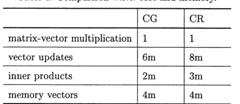
the conjugate residual method (CR hereafter).

Table 1 shows

a

comparison between CG and CR with respect to computa-tional costs at each iteration and memory.

Table 1. Comparison w.r.t. cost and memory.

Although CR is expensive than CG with respect to vector updates and inner products at each iteration, the total computat,ionalcosts during each iteration

in CG and CR

are

almost equalbecause the dense matrix-vectormultiplication is the major part. Fewer iterations to achieve the stopping criterion

means

better performance ofconvergence.

4 Numerical experiments

In this section,

we

report several numerical experiments to compare the

com-putational performance between CG and $\mathrm{C}\mathrm{R}$. All experiments have been

car-ried out with double precision floating point arithmetic

on an

Alpha computer ($750\mathrm{M}\mathrm{H}_{\mathrm{Z})}$. We always $\mathrm{c}\mathrm{h}_{\mathrm{o}\mathrm{O}\mathrm{S}}\mathrm{e}$ the initial guess

$x_{0}=0$ in ALGORITHM 1 and ALGORITHM 2. Allfigures throughout this section display the logarithmic rela-tive residual 2-norm $\log_{10}||r_{i}||/||r_{0}||$ (on the vertical axis)

versus

the iteration

number $i$ (on the horizontal axis).

Here

we

consider a Maximum Clique problem. Here all data in (1)

are

given

as

follows: $A_{0}$ is the matrix whose all elements

are

equal to 1, $A_{1}$ is the identity

matrix, $A_{l}$ $(l=2, \cdots , m)$ is

a

matrix in which the ij-th andji-th elements

are

equal to $-1$ for

a

given integer pair _{$(i,j)(1\leq i<j\leq n)$} and else elements

We applied the interior-point method to

a

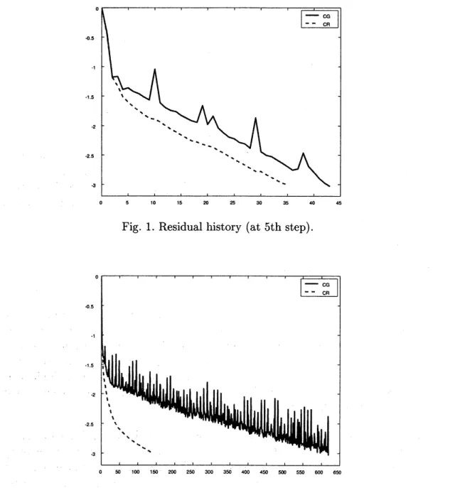
Maximum Clique problem and its dual problem simultaneously with $m=9957$ and $n=200$. The following two

figures show the numerical results of CG

versus

CR for solving SDP’s linear

systems at 5th step and 10th step in the interior-point method respectively. The stopping criterion is set

as

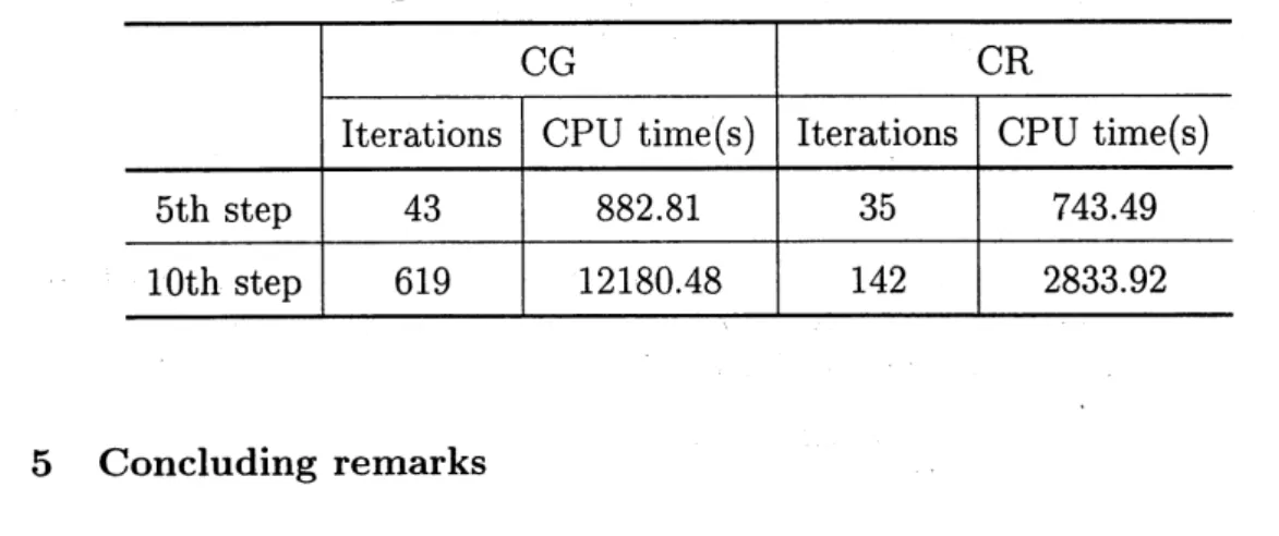
$10^{-3}$. Table 2 $\mathrm{s}h$

ows

the performance for CG

and

CR

in terms of the total numbers of iterations and CPU times to achieve

the stopping criterion. Throughout the Maximum Cliqueproblem,

we

suppose

deliberately that the all elements ofthe matrix$B$ in (2)

can

be not kept

simul-taneously in the memory of the computer. To compute $Bp_{i}$ in ALGORITHM 1

and

ALGORITHM

2, the element $B_{ij}$ is computed extemporaneously via (3) at

each iterative step. Note that the computation of $Bp_{i}$ costs very much, then

takes most ofCPU time.

Fig. 1. Residualhistory (at 5th step).

We observe that

CR

began to

converge

faster than

CG

at 5th step from Fig. 1 and Table 2. At 10th step where the approximate solution (X,$y,$ $Z$) in the interior-point method

was

very close to the optimal solution,

we

had to solve

an

ill-posed matrix $B$ because $X$ and $Z$ became numerically nearly singular.

From Fig. 2 and Table 2,

we

observe that CR became

more

efficient and

more

useful for this difficult one. Therefore, it

can

be said that CR is suitable for the Maximum Clique problem.

Table 2. $\mathrm{T}11\mathrm{e}$ performance for the Maximum Clique problem.

5 Concluding remarks

In the present paper,

we

considered the application of GCR to the large and dense line$a\mathrm{r}$ systems which arise from Semidefinite Programming. Comparing

the theoretic$a1$ aspect of CG and GCR, we emphasize that GCR has

some

$at$tractive and competitive features for solving SDP’s linear systems. The

nu-merical experiments showed that GCR is suitable and powerful for solving

SDP’s linear systems.

References

[1] F. Alizadeh, J.-P. A. Haeberly and M. L. Overton, Primal-dual

interior-point methods

_for

_semidefinite

programming: convergence rates, stability and

numerical results, SIAM J. Optim., 8 (1998) 746-768.

[2] B. Borchers, CSDP 2.3 user’s guide, Optimization Methods and Software,

11-12 (1999) 597-611.

[3] S. C. Eisenstat, H. C. Elman and and M. H.Schultz, Variational Iterative

Methods

_for

Nonsymmetric Systems

_of

Linear Equations, SIAM J. Numer.

Anal., 20 (1983) 345-357.

[4] K. Fujisawa, M. Kojima and K. Nakata, SDPA (Semidefinite Programming

Algorithm) - user’s manual -, (Technical Report B-308, Department of

[5] K. Fujisawa, M. Fukuda, M. Kojima and K. Nakata, Numerical evaluation

_of

SDPA (SemiDefinite Programming Algorithm), in: H. Frenk el at.,eds, High

Performance Optimization, (Kluwer Academic Publishers, 1999) 267-301.

[6] C. Helmberg, F. Rendl, R. J. Vanderbei and H. Wolkowicz, An interior-point

method

_for

_semidefinite

programming, SIAM J. Optim., 6 (1996) 342-361.

[7] M. R. Hestenes and E. Stiefel, Methods

_of

conjugate gradients

_for

solving linear

systems, J. Res. Nat. Bur. Standards, 49 (1952) 409-435.

[8] E. F. Kaasschieter, Preconditioned conjugate gradients

_for

solving singular

systems, J. Comput. Appl. Math., 24 (1988) 265-275.

[9] M. Kojima, S. Shindoh and S. Hara, Interior-point methods

_for

the monotone

semidefinite

linear complementarity problems, SIAM J. Optim., 7 (1997)

86-125.

[10] C. Lin and R. Saigal, Onsolving large-scale

_semidefinite

programming

problems-a cproblems-ase study

_of

quadratic assignment problem, (Technical report, Department

of Industrial and Operations Engineering, University of Michigan, 1998).

[11] R. D. C. Monteiro, Primal-dual path-following algorithms

_for

_semidefinite

programming, SIAM J. Optim., 7 (1997) 663-678.

[12] R. D. C. Monteiro and Y. Zhang, A

_unified

analysis

_for

a class

_of

path-following primal-dual interior-point algorithms

_for

_semidefinite

programming,

Math. Programming, 81 (1998) 281-299.

[13] K. Nakata, K. Fujisawa and M. Kojima, Using the conjugate gradient method

in interior-point methods

_for

_semidefinite

programs (in Japanese), Proceedings

of the Institute of Statistical Mathematics, 46 (1998) 297-316.

[14] F. A. Potra, R. Sheng and N. Brixius, SDPHA -a MATLAB implementation

of

homogeneous interior-point algorithms

_{for semidefinite}

programming,

(Department ofMathematics, University of Iowa, 1997).

[15] K. C. Toh, M. J. Todd and R. H. T\"ut\"unc\"u, SDPT3 -a MATLAB

_software

package

_for

_semidefinite

programming, (Dept. of Mathematics, National

University ofSingapore, 1996).

[16] L. Vandenberghe and S. Boyd,

_Semidefinite

programming, SIAM Rev., 38

(1996) 49-95.

[17] S.-L. Zhang, Y. Oyanagi and M. Sugihara, Necessary and

_Sufficient

Conditions

for

Convergence

_of

$\mathrm{O}rth_{\mathit{0}}\min(k)$ on Singular and Inconsistent Linear Systems,

Numer. Math., 87-2 (2000) 391-405.

[18] Q. Zhao, S. E. Karisch, F. Rendl and H. Wolkowicz,

_Semidefinite

programming

relaxation

_for

the quadratic assignment problem, (CORR Report 95-27,