Solvability of the initial value problem to a model system for water waves (Recent Advances on Mathematical Aspects of Nonlinear Wave Phenomena)

(1)

Solvability of the

initial

value problem

to

a

model system

for

water

waves

慶慮義塾大学理工学部数理科学科井口達雄(Tatsuo Iguchi)

Department ofMathematics, Faculty of

Science

and Technology,

Keio University

1 Introduction

Thewater

wave

problemismathematicallyformulated

as

a

free boundary$p_{1}\cdot$oblem for

an

irrotational flow of

an

inviscid and incompressiblefluid under thegravitational field. The

basic equations for water

waves are

complicated due to the nonlinearity of the equations

together with the presence of

an

unknown free surface. Therefore, until

now

many

ap-proximateequationshavebeen proposed and analyzed to understand natul.al phenomena

for water

waves.

Famous examples of such approximate equations

are

the shallow

wa-ter equations, the Green-Naghdi equations, Boussinesq type equations, the Korteweg-de

Vriesequation, theKadomtsev Petviashviliequation, the Benjamin Bona-Mahony

equa-tion, the Camassa-Holm equation, the Benjamin-Ono equations, and so

on.

All of them

are

derived from the water

wave

problem under the shallowness assumptionof the water

waves, which

means

that the

mean

depth of the water is suﬃciently small compared to

the typical wavelength ofthe water surface.

On the other hand, in coastal engineering

some

model equationswerederived without

using any shallowness aesumI)tion of the water

waves.

It is well-known that the water

wave

problem has a variational structure. In fact, J. C. Luke [7] gave

a

Lagrangian in

termsofthe velocitypotential $\Phi$and thesurfacevariation

$\eta$

.

His Lagrangianhastheform

(1.1) $\mathscr{L}(\Phi, \eta)=\int_{b(x\rangle}^{h+\eta(x,t)}(\Phi_{t}(x, z,t)+\frac{1}{2}|\nabla_{x,z}\Phi(x, z,t\rangle|^{2}+g(z-h))dz$

and the action function is

$\mathscr{J}(\Phi,\eta)=\int_{t_{0}}^{t}/\Omega^{\mathscr{L}(\Phi,\eta)dxdt}$

’

where $g$ is the gravitational constant, $h$ is the

mean

depth of the water, $b$represents the

bottom topography, and $\Omega$

is

an

appropriate region in $R^{n}$

.

In view ofBernoulli’s law $($1.2$)$ $\Phi_{i}+\frac{1}{2}|\nabla_{x,z}\Phi|^{2}+\frac{1}{p}(p-Po)$ 牽$g(z-h)\equiv 0,$

(2)

we

see

that Luke’s

Lagrangian is essentially

the

integral

of

the pressure$p$ in the

vertical

direction of the water region. J. C. Luke showed that the corresponding Euler-Lagrange

equationis exactly the basicequations for water

waves.

M. Isobe [2, 3] and T. Kakinuma

[4, 5, 6] used this variational structure of the water

waves

to derive approximate model

equations. They approximated the velocity potential in $Luke^{\rangle}s$ Lagrangian

as

$\Phi(x, z, t)\simeq\sum_{k=0}^{K}\Psi_{k}(z;b)\phi^{k}(x, t)$,

where $\{\Psi_{k}\}$is

an

appropriatefunction system, and derived

an

approximateLagrangianfor

$(\eta, \phi^{0}, \phi^{1}, \ldots, \phi^{K})$

.

Their model equations

are

the corresponding Euler Lagrange

equa-tions.

There

are

several choices of thefunction system $\{\Psi_{k}\}$

.

As

was

shown byJ. Boussinesq

[1], in the

case

of the flat bottom the velocity potential $\Phi$

can

be expanded in

a

Taylor

series with respect to the vertical spatial variable

as

$\Phi(x_{\sim}^{\gamma}, t)=\sum_{k=0}^{\infty}\frac{z^{2k}}{(2k)!}(-\Delta)^{k}\phi_{0}(x, t)$,

where $\phi_{0}$ is the trace of the velocity potential $\Phi$ on the bottom. Therefore,

one

of the

choice of the approximation

was

given by

(1.3) $\Phi(x, z, t)\simeq\sum_{k=0}^{K}(z-b(x))^{2k}\phi^{k}(x, t)$

.

In the

case

$K=0$, that is, if we

use

the approximation $\Phi(x, z, t)\simeq\phi^{0}(x, t)$ in $Luke^{\rangle}s$

Lagrangian, then the Lagrangian (1.1) is approximated by

$\mathscr{L}(\phi^{0}, \eta)=\int_{b(x)}^{h+\eta(x,t)}(\phi_{t}^{0}+\frac{1}{2}|\nabla\phi^{0}|^{2}+g(z-h))dz$

$=( \phi_{t}^{\mathfrak{o}}+\frac{1}{2}|\nabla\phi^{0}|^{2})(h+\eta-b)+\frac{1}{2}9(\eta^{2}-(b-h)^{2})$

.

The corresponding Euler-Lagrangeequations

are

exactly the shallow water equations.

$\{\begin{array}{l}\eta_{t}+\nabla\cdot((h+\eta-b)\nabla\phi)=0,\phi_{t}+\frac{1}{2}|\nabla\phi|^{2}+g\eta=0.\end{array}$

In the

case

$K=1$, that is, ifwe

use

the approximation

(3)

in Luke’s Lagrangian, thenthe Lagrangian (1.1) is approximated by

$\mathscr{L}(\phi^{0}, \phi^{1}, \eta)=H\phi_{t}^{0}+\frac{1}{3}H^{3}\phi_{t}^{1}$

$+ \frac{1}{2}H|\nabla\phi^{0}|^{2}+\frac{1}{10}H^{5}|\nabla\phi^{1}|^{2}+\frac{2}{3}H^{3}(1+|\nabla b|^{2})(\phi^{1})^{2}$

$+ \frac{1}{3}H^{3}\nabla\phi^{\mathfrak{o}}\cdot\nabla\phi^{1}-H^{2}\phi^{1}\nabla b\cdot\nabla\phi^{0}-\frac{1}{2}H^{4}\phi^{1}\nabla b\cdot\nabla\phi^{1}$

$+ \frac{1}{2}g(\eta^{2}-(b-h\rangle^{2})$,

where $H=H(x, t)=h+\eta(x, t)-b(x)$ is the depth at the point $x$ at time $t$

.

The

corresponding Euler-Lagrange equations have the form

(1.5) $\{\begin{array}{l}\eta_{t}+\nabla\cdot(H\nabla\phi^{0}+\frac{1}{3}H^{3}\nabla\phi^{1}-H^{2}\phi^{1}\nabla b)=0,H^{2} 恥 +\nabla\cdot(\frac{1}{3}H^{3}\nabla\phi^{0}+\frac{1}{8}H^{s}\nabla\phi^{1}-\frac{1}{2}H^{4}\phi^{1}\nabla b)+H^{2}\nabla b\cdot\nabla\phi^{0}+\frac{1}{2}H^{4}\nabla b\cdot\nabla\phi^{1}-\frac{4}{3}H^{3}(1+|\nabla b|^{2})\phi^{1}=0,\phi_{t}^{0}+H^{2}\phi_{t}^{1}+g\eta+\frac{1}{2}|\nabla\phi^{0}|^{2}+\frac{1}{2}H^{4}|\nabla\phi^{1}|^{2}+H^{2}\nabla\phi^{0}\cdot\nabla\phi^{1}-2H\phi^{1}\nabla b\cdot\nabla\phi^{0}-2H^{3}\phi^{1}\nabla b\cdot\nabla\phi^{1}+2H^{2}(1+|\nabla b|^{2})(\phi^{1})^{2}= O.\end{array}$

This isone ofthemodelproposed by M. Isobe and T. Kakinuma. In thiscommunication,

we

reportthe solvability oftheinitialvalue problemforthis Isobe-Kakinumamodal under the initial conditions

(1.6) $(\eta, \phi^{0}, \phi^{1})=(\eta_{0}, \phi_{0}^{0}, \phi_{0}^{1})$ at $t=0.$

2 Basic

properties

of

the

model

The linearized equations ofthe $Isobe\frac{-}{}$Kakinumamodel (1.5) around the trivial flow

are

$\{\begin{array}{l}\eta_{t}+h\Delta\phi^{0}+\frac{}{}\Delta\phi^{1}=0\eta_{t}+\frac{h}{3}\triangle\phi^{0}+\frac{h^{3}h^{3}3}{5}\Delta\phi^{1}-\frac{4}{3}h\phi^{1}=0,\phi_{t}^{0}+h^{2}\phi_{t}^{1}+g\eta=0.\end{array}$

This system has

a

non-trivial solution of the form $\eta(x, t)=\eta_{0}e^{i(\xi\cdot x-\omega t)}$ if and only if the

wave

vector$\xi\in R^{n}$ and the angular frequency $(Jj\in C$ satisfy the relation

(4)

This is the linear dispersion relation for the Isobe-Kakinuma model (1.5),

so

that the

phase speed $c_{IK}= \frac{\omega}{|\zeta|}$ is givenby

$c_{IK}(\xi)=\pm\sqrt{gh\frac{1+\frac{1}{15}h^{2}|\xi|^{2}}{1+\frac{2}{5}h^{2}|\xi|^{2}}}.$

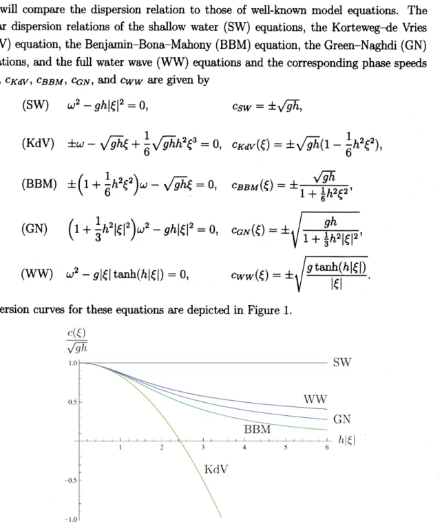
We will compare the dispersion relation to those of well-known model equations. The

linear dispersion relations of the shallow water (SW) equations, the Korteweg-de Vries

$(KdV)$ equation,

the

Benjamin

Bona

_{Mahony (BBM)} _equation, _{the Green-Naghdi} _(GN)

equations, and the full water

wave

(WW) equations and the corresponding phase speeds

$c_{SW},$ $c_{KdV},$ $c_{BBM},$ $c_{GN}$, and $c_{WW}$

are

given by

(SW) $\omega^{2}-gh|\xi|^{2}=0,$ $c_{SW}=\pm\sqrt{gh},$

$( KdV) \pm\omega-\sqrt{gh}\xi+\frac{1}{6}\sqrt{gh}h^{2}\xi^{3}=0, c_{KdV}(\xi)=\pm\sqrt{gh}(1-\frac{1}{6}h^{2}\xi^{2})$,

(BBM) $\pm(1+\frac{1}{6}h^{2}\xi^{2})\omega-\sqrt{gh}\xi=0,$ $c_{BBM}( \xi)=\pm\frac{\sqrt{gh}}{1+\frac{1}{6}h^{2}\xi^{2}},$

(GN) $(1+ \frac{1}{3}h^{2}|\xi|^{2})\omega^{2}-gh|\xi|^{2}=0,$ $c_{GN}(\xi)=\pm\sqrt{\frac{gh}{1+\frac{1}{3}h^{2}|\xi|^{2}}},$

(WW) $\omega^{2}-g|\xi|\tanh(h|\xi|)=0,$ $c_{WW}(\xi)=\pm\sqrt{\frac{gtmh(h|\xi|)}{|\xi|}}.$

Dispersion

curves

for these equations

are

depicted in Figure 1.

$\frac{c(\xi)}{\sqrt{g}\hslash}$

(5)

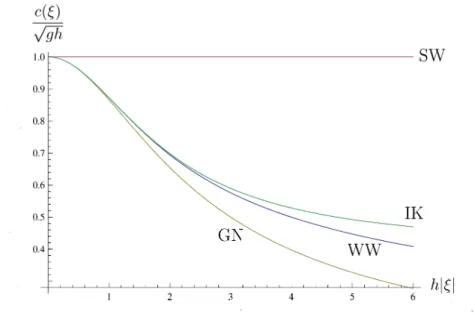
Among these model equations, the Green-Naghdi equations give the best approximation

in the shallow water regime $h|\xi|\ll 1$. Now, let

us

compare the dispersion

curves

for the

Green-Naghdi equations and the Isobe-Kakimuma (IK) model.

Figure 2: Dispersion

curves

for SW, GN, IK, and WWequations

In view of Figure 2,

we

see that the Isobe-Kakinumamodel gives a much better

approx-imation than the Green-Naghdi equations in the shallowwater regime. Mathematically,

we

can

characterize

a

relation of these approximations

as

follows.

$(KdV)$ $c_{KdV}( \xi\rangle=\pm\sqrt{gh}(1-\frac{1}{6}h^{2}\xi^{2})=Tay1\circ r$ approximationof $c_{WW}(\xi)$,

(BBM) $c_{BBM}( \xi)=\pm\frac{\sqrt{gh}}{1+\frac{1}{6}h^{2}\xi^{2}}=[0/2]$ Pad6 approximant of $c_{WW}(\xi)$,

(GN) $(c_{GN}( \xi))^{2}=\frac{gh}{1+\frac{\ddagger}{3}h^{2}|\xi|^{2}}=[0/2]$ Pad\’e approximant of $(c_{WW}(\xi))^{2},$

(IK) $(c_{IK}( \xi))^{2}=gh\frac{1+\frac{1}{16}h^{2}|\xi|^{2}}{1+\frac{2}{5}h^{2}|\xi|^{2}}=[2/2]$ Pad\’e approximant of $(c_{WW}(\xi))^{2}$

Therefore, the Isobe-Kakinumamodel (1.5) gives a very good approximation in the

shal-low water regime at least in the linear level.

It is weil known that the fun water wave problem has a conserved energy $E_{WW}(t)$,

which is the

sum

of the kinetic and potential energies and given by

$E_{WW}(t)= \frac{\rho}{2}\int_{R^{n}}\{\int_{b\langle x\rangle}^{\hslash+\eta\langle x,t)}|\nabla_{x,z}\Phi(x, z, t)|^{2}dz+g(\eta(x, t))^{2}\}dx.$

(6)

$E_{IK}(t)$ for the Isobe-Kakinuma model (1.5)

$E_{IK}(t)= \frac{\rho}{2}\int_{R^{n}}\{\int_{b(x)}^{h+\eta(x,t)}|\nabla_{x,z}(\phi^{0}(x, t)+(z-b(x))^{2}\phi^{1}(x, t))|^{2}dz+g(\eta(x, t))^{2}\rangle dx.$

It is easy to show that this is

a

conserved quantity for smooth solutions to the

Isobe-Kakinuma model (1.5).

The Isobe-Kakinuma model (1.5) is written in the matrix form

as

$(\begin{array}{lll}1 0 0H^{2} 0 00 1 H^{2}\end{array})\frac{\partial}{\partial t}(\begin{array}{l}\phi^{0}\eta\phi^{1}\end{array})+$

{

spatial

_derivatives}

$=0.$

Since thecoeﬃcient matrix always has the

zero

eigenvalue, the hypersurface $t=0$ _{in the}

space-time $R^{n}\cross R$is characteristic for the model,

so

that the initial _{value problem (1.5)}

and (1.6) is not solvable in general. In fact, if the problem hasa solution $(\eta, \phi^{0}, \phi^{1})$, then

by eIiminating the time derivative $\eta_{t}$ from the first two equations in (1.5) we

see

that the

solution has to satisfy therelation

$H^{2} \nabla\cdot(H\nabla\phi^{0}+\frac{1}{3}H^{3}\nabla\phi^{1}-H^{2}\phi^{1}\nabla b)$

(2.2) $= \nabla\cdot(\frac{1}{3}H^{3}\nabla\phi^{\mathfrak{o}}+\frac{1}{5}H^{5}\nabla\phi^{1}-\frac{1}{2}H^{4}\phi^{1}\nabla b)$

$+H^{2} \nabla b\cdot\nabla\phi^{0}+\frac{1}{2}H^{4}\nabla b\cdot\nabla\phi^{1}-\frac{4}{3}H^{3}(1+|\nabla b|^{2})\phi^{1}.$

Therefore,

as

a necessarycondition the initial date $(\eta_{0}, \phi_{0}^{0}, \phi_{0}^{1})$ andthe bottom topography

$b$have to satisfy the relation (2.2) for the existence of

the solution,

3

Main

result

Beforegiving

our

mainresultwenote

a

generalized Rayleigh-Taylor sign condition for the

fullwater

wave

problem. It is known that the well-posedness of the initial value problem

for the full water

wave

equations may be broken unless the following sign condition is

satisfied.

-$\frac{\partial p}{\partial N}\geq c_{0}>0$ on the water surface,

where$p$is the pressure and $N$ is the unit outward normal to the water surface. Since _$p$

is constanton the water surface, this condition is equivalent to the condition

-$\frac{\partial p}{\partial z}\geq c_{0}>0$ on the water surface.

Now,

we

define a function $a=a(x, t)$ by

(3.1) $a:=g+2H\phi_{t}^{1}+2H^{3}|\nabla\phi^{1}|^{2}+2H\nabla\phi^{0}\cdot\nabla\phi^{1}-2\phi^{1}\nabla b\cdot\nabla\phi^{0}$

(7)

Then, in view of Bernoulli’s law (1.2) and our approximation (1.4),

we

have

-$\frac{\lambda}{\rho}\partial_{z}p=$

$g+\partial_{z}\Phi_{t}+\nabla_{X}\partial_{z}\Phi\cdot\nabla_{X}\Phi=a$

on

the water surface. Therefore, it is natural to

assume

that this function $a$ is positive definite at the initial time $t=$ O. We also remark that

we can express the term $\phi_{t}^{I}(x,$$0\rangle$ in $a(x,$$0\rangle$ in terms of the initial data and $b$ although

the hypersurface $t=0$ is characteristic. Let $H^{m}$ be the Sobolev space of order $m$

on

$R^{n}$

equipped with a norm $\Vert\cdot\Vert_{\uparrow n}$

.

The following is ourmain theorem in this communication.

Theorem 3.1 ([8]). Let $g,$ $h,$$c_{0},$$M_{0}$ be positive constants and $m$

an

integer such that

$m> \frac{n}{2}+1$

.

There exists

a

time $T>0$ such that

if

the initial data $(\eta_{0}, \phi_{0}^{0}, \phi_{0}^{1})$ and$b$ satisfy

the relation (2.2) and

(3.2) $\{\begin{array}{l}\Vert\eta_{0}\Vert_{m}+\Vert\nabla\phi_{0}^{0}\Vert_{m}+\Vert\phi_{0}^{1}\Vert_{m+1}+\Vert b\Vert_{W^{m+2,\infty}}\leq M_{0},h+\eta_{0}(x)-b(x)\geq c_{0_{7}} a(x, 0\rangle\geq c_{0} for x\in R^{n},\end{array}$

then the initial valueproblem (1.5) and (1.6) has a unique solution $(\eta,$$\phi^{0},$$\phi^{1}\rangle$ satisfying

$\eta,$$\nabla\phi^{0}\in C([0, T];H^{m})$, $\phi^{1}$ 欧 $C([0, T H^{rn+1})$

.

Theidea to prove this theoremis sosimple. Wetrax)sform_the _{Isobe-Kakinuma}_model

$(1.5\rangle$ to a system of equations for which the hypersurface $t=0$ is noncharacteristic by

using the necessary condition (2.2). In fact, diﬀerentiating the necessary condition (2.2)

with respect to time $t$and using thefirst (orthe second) equation in (1.5) to eliminate $\eta_{t}$

we

obtain

$H^{2} \nabla\cdot(H\nabla\phi_{t}^{0}+\frac{1}{3}H^{3}\nabla\phi_{i}^{1}-H^{2}\phi_{t}^{1}\nabla b)$

$= \nabla\cdot(\frac{1}{3}H^{3}\nabla\phi_{t}^{0}+\frac{1}{5}H^{5}\nabla\phi_{t}^{1}-\frac{1}{2}H^{4}\phi_{t}^{1}\nabla b)$

$+H^{2} \nabla b\cdot\nabla\phi_{t}^{0}+\frac{1}{2}H^{4}\nabla b\cdot\nabla\phi_{t}^{1}-\frac{4}{3}H^{3}(1+|\nabla b|^{2})\phi_{t}^{1}+$

{

spatial

derivatives}.

This together with the third equation in (1.5) gives evolution equations for $\phi^{0}$ and $\phi^{1}.$

We superimpose thefirstand the second equation in (1.5) to derive

an

evolution equation

for $\eta$ in order that the resulting system of equations has a good symnletric structure. In

such a way we

can

derive the following system ofequations.

(8)

where$a$isdefinedby (3.1), $f_{1},$$f_{2},$$f_{3}$

are

collections

of lowerorder terms and do not include

any time derivatives, and $a_{0},$$a_{1},$$u$

are

given by

$\{\begin{array}{l}a_{0}:=\frac{15}{2}H^{-1}\{\frac{4}{3}(1+|\nabla b|^{2})+2\nabla b\cdot\nabla H+\frac{8}{3}|\nabla H|^{2}+\frac{2}{3}H\Delta H-\frac{1}{2}H\Delta b\},a_{1}:=\frac{3}{2}H^{3}\{\frac{4}{3}(1+|\nabla b|^{2})+2\nabla b\cdot\nabla H-\frac{4}{3}|\nabla H|^{2}-\frac{4}{3}H\Delta H-\frac{1}{2}H\Delta b\},u:=\nabla\phi^{\mathfrak{o}}+H^{2}\nabla\phi^{1}-2H\phi^{1}\nabla b.\end{array}$

We

can

rewrite (3.3) in the matrix form

as

$(\begin{array}{lll}a_{0}-\nabla\cdot 4H^{5}\nabla 0 00 a_{1}-\nabla\cdot\frac{4}{5}H\nabla 00 0 a\end{array})\frac{\partial}{\partial t}(\begin{array}{l}\phi^{0}\phi^{l}\eta\end{array})$

$+(0 - \nabla\cdot((.\frac{4}{5}H^{5}u\cdot\nabla)\nabla\nabla a_{2}H^{3}\nabla 0 -\nabla aH^{3}\nabla\nabla\cdot.aH\nabla 9au\cdot\nabla)(\begin{array}{l}\phi^{0}\phi^{1}\eta\end{array})=F.$

It is easy to

see

that the matrix operator in the second term in the left hand side is

skew-symmetric in $L^{2}$

modulo lower order terms, so that once we show the positivity

of the functions $a_{0}$ and $a_{1}$

we see

that the matrix operator in the first term behaves

a

symmetrizer. Oncewe find

a

symmetrizer,

we

can

define

a

mathematicalenergy function

and derive

an

energy estimate, whichleads to the existenceof the solution for the initial

valueproblemto the reduced system (3.3). Tothisend,

we

show thefollowingkey lemma.

Lemma 3.1 Supposethat$0<c_{0}\leq H(x)\leq c_{1}$ and$\nabla b\in L^{\infty}(R^{n})$

.

There exists

a

positive

constant $C=C(c_{\theta}, c_{1})$ depending only

on

$c_{0}$ and $c_{1}$ such that

we

have

$\{\begin{array}{l}((a_{0}-\nabla\cdot 4H^{5}\nabla)\psi^{0}, \psi^{0})_{L^{2}}\geq C^{-1}\Vert\psi^{0}\Vert_{1}^{2},((a_{1}-\nabla\cdot\frac{4}{5}H\nabla)\psi^{1}, \psi^{1})_{L^{2}}\geq C^{-1}\Vert\psi^{1}\Vert_{1}^{2}.\end{array}$

Thanks to this lemma, under physically reasonable conditions

on

the initial data

to-gether with the sign condition,

we

can

prove the solvability ofthe initial value problem

for the reduced system (3.3) and (1.6). Herewedo notneed the necessary condition(2.2).

Finally, we have to show that the solution satisfies the original Isobe-Kakinuma model

(1.5) under the condition (2.2). We refer to [8] for the details.

References

[1] J. Boussinesq, Th\’eorie des ondes et des

remous

qui

se

propagent le long d’un canal

rectangulaire horizontal, en communiquant au liquide contenu dans

ce

canal des

vitesses sensiblementpareillesde la surfaceaufond, J. Math. Pure. Appl., 17 (1872),

(9)

[2] M. Isobe, A proposal

on a

nonlinear gentle slope

wave

equation, Proceedings of

Coastal Engineering, Japan Society of Civil Engineers, 41 (1994), 1-5 [Japanese].

[3] M. Isobe, Time-dependent mild-slope equations for random waves, Proceedings of

24th International Conference

on

Coastal Engineering, ASCE, 285-299, 1994.

$[4]\prime r$

.

Kakinuma, [title in Japanese], Proceedings of CoastalEngineering, Japan Society

of Civil Engineers, 47 (2000), 1-5 [Japanese].

[5] T. Kakinuma, A set of fully nonlinear equations for surface and internal gravity

waves, Coastal Engineering V: Computer Modelling of Seas and Coastal Regions,

225-234, WIT Press, 2001.

[6] T. Kakinuma, Anonlinear numerical modelfor surfaceand internal

waves

shoaling

on

apermeable beach, Coastal engineering VI: Computer Modelling and Experimental

Measurements ofSeas and Coastal Regions, 227-236, WIT Press,

2003.

[7] J. C. Luke,

A

variationalprinciple for

a

flu\’id with

a

free surface, J. Fluid Mech., 27

(1967), 395-397.

[8] Y. Murakami andT. Iguchi, Solvability of the initialvalueproblemtoamodel system