JAXA Research and Development Report
February 2018
Japan Aerospace Exploration Agency
Guidance Law Based on Real-time Trajectory Prediction for
D-SEND#2
1
Introduction ··· 2
2
Guidance Law ··· 4
2.1 Overview ··· 4
2.2 Acceleration Phase ··· 5
2.3 Pull-up Phase ··· 5
2.4 Glide Phase ··· 6
2.5 Dive Phase ··· 6
2.6 Measurement Phase ··· 9
3
Evaluation of Performance ··· 9
3.1 Presumed Conditions ··· 9
3.2 Error Models ··· 10
3.3 Monte Carlo Simulation (MCS) ··· 10
4
Result of Actual Flight ··· 12
4.1 Actual Flight Trajectory ··· 12
4.2 Conputational Load on On-board Flight Computer ··· 13
4.3
Acceptance for Required Conditions ··· 13
4.4
Results of Real-Time Trajectory Prediction Method ··· 14
By
Hirokazu SUZUKI
*1and Tetsujiro NINOMIYA
*2Abstract: A flight experiment using a stratospheric balloon, designated as D–SEND#2, was carried out in 2015. This paper describes a guidance law of the D–SEND#2 vehicle. A typical
problem of flight experiment using a stratospheric balloon is that it has no nominal trajectory.
Therefore, a new real-time trajectory prediction method is devised to overcome this problem.
The method solves equations of motion directly for various load factor commands. The guidance
law was evaluated using Monte Carlo simulation, and its result was the success rate of 98.1%.
The guidance law has a little tolerance to the uncertainty of steady wind and of the model
error of CD because the vehicle has no engine nor devices for velocity control. Actual flight experiments demonstrated that the guidance law satisfied all mission requirements and that it
contributed greatly to the mission success.
Keyword: Guidance and Control, Real-time, Trajectory Prediction, D–SEND
Nomenclature
Nz : Load factor
CL, CD : Lift and drag coefficient
CN : Normal force coefficient
G DP1,G GM2 : Guidance parameter G RG3,G h4 : Guidance parameter G N z4,G RG4 : Guidance parameter
L, D : Lift and drag
R : Range
Ts : Time constant for a angle of attack response model
V : Velocity
doi: 10.20637/JAXA-RR-17-010E/0001 *
Received January 30, 2017 *1
X4F : Final flight conditions in phase 4
X5I : Initial flight conditions in phase 5
g : Gravitational acceleration
h : Altitude
m : Vehicle mass
r : A radius from the center of the Earth to the center of gravity of the vehicle
α : Angle of attack
αi : Angle of attack command for phase i
γ : Flight path angle
Subscripts
c : Command
1
Introduction
The Japan Aerospace Exploration Agency (JAXA) has conducted a Drop test for Simplified Evaluation of Non-symmetrically Distributed sonic boom (D–SEND) to verify the low boom design using computational fluid dynamics. D–SEND comprises two series of balloon drop tests: D–SEND#1 and D–SEND#21). For D–
SEND#1, an uncontrolled symmetric vehicle was dropped. Then, a controlled experimental low-boom airplane was dropped in D–SEND#2. Both small vehicles achieved supersonic flight without an engine.
Figure 1 presents the D–SEND#2 vehicle configuration. Figure 2 portrays an outline of the flight experiment. The vehicle is dropped from an altitude of 30 km from a stratospheric balloon. The vehicle uses gravity to accelerate to supersonic and passes over a microphone which measures a sonic boom. The measurement system with the microphone for a sonic boom is designated as the Boom Measurement System (BMS)2). The microphone
is moored at an altitude of 1 km using a captive balloon to measure the sonic boom, which is not disturbed by
単位[mm]
7913(スタビレータ舵角0°時)
35
10
FSTA 1000
BL 0
FSTA WL BL
WL
172
WL 2000
Reference area 4.891 m2 Chord 1.912 m
Span 3.510 m
172mm
3
5
1
0
m
m
7913mm
Fig. 2 Summary of flight experiment.
turbulence near the ground.
Only two flight experiments have used a stratospheric balloon for an unmanned supersonic vehicle with
guidance and control: the Japanese High-Speed Flight Demonstrator phase–II (HSFD–II)3) in 2003 and the
Italian Unmanned Space Vehicle (USV)4) in 2010. The main objectives of these flight experiments were the
measurement of its aerodynamic characteristics by an α-sweep maneuver for maintaining the Mach number
during flight. The position for measurement was not prescribed because measurements were taken by on-board
sensors.
The main objective of D–SEND#2 is to measure a sonic boom by the BMS from the ground. Because the
stratospheric balloon has no device for controlling its position within the horizontal plane, one BMS is selected
from three BMSs set up in the flight test area after the separation. Therefore, the vehicle must establish a
desirable flight condition above the BMS from the separation point, which cannot be prescribed beforehand.
Hence, the vehicle must satisfy both requirements of flight conditions above the BMS and those of precise
guidance for the BMS position at the same time.
This paper presents a specific examination of a guidance law of D–SEND#2 vehicle. The most important
requirements for the guidance law are the following.
A) The guidance law must be processed by an on-board computer within a 10 Hz cycle.
B) The guidance law must adjust to an extremely wide separation space because the separation position can
not be prescribed.
C) The guidance law has no nominal trajectory. Therefore, even if a proper flight trajectory does not exist
in the actual flight, the guidance law must output some preferred commands.
The guidance law comprises two main logics to adjust those requirements. The first logic outputs some
named as reference trajectories. The second logic is devised to overcome B) and C). It is based on a real-time
trajectory prediction. The method obtains various trajectories from solving the equations of motion directly
by inputting the load factor command as a parameter. The method selects the most desirable trajectory from
them. Solving the equations of motion overcomes C). It has another benefit: constraints such as dynamic
pressure or load factor can be dealt with directly. When the trajectory does not meet with those constraints,
it is rejected. If all the trajectories do not satisfy the requirements, then the most preferred trajectory can be
selected.
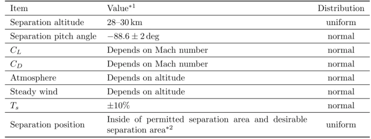
The Esrange Space Center in Sweden was selected as the flight experiment site. Because the BMS must be
set on the ground, other candidates were rejected. The flight test field is designated as Zone B (see Fig. 7).
2
Guidance Law
2.1
Overview
Measurement requests of flight conditions at the sonic boom generation are presented in Table 1. Constraints
for flight trajectory are the followings.
• Dynamic Pressure<65 kPa
• Load Factor<4.5 G
The guidance law must satisfy the measurement requests and the constraints of actual flight. The guidance
law comprises two logics. The first logic outputs the guidance commands based on the trajectory data to the
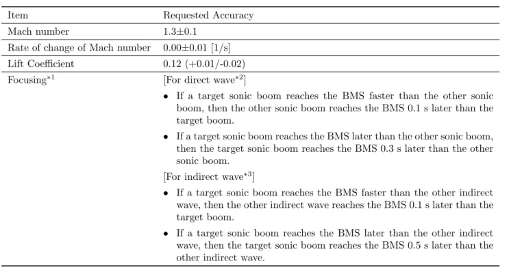
Table 1 Requirements for sonic boom measurement.
Item Requested Accuracy
Mach number 1.3±0.1
Rate of change of Mach number 0.00±0.01 [1/s]
Lift Coefficient 0.12 (+0.01/-0.02)
Focusing∗1 [For direct wave∗2]
• If a target sonic boom reaches the BMS faster than the other sonic
boom, then the other sonic boom reaches the BMS 0.1 s later than the target boom.
• If a target sonic boom reaches the BMS later than the other sonic boom,
then the target sonic boom reaches the BMS 0.3 s later than the other sonic boom.
[For indirect wave∗3
]
• If a target sonic boom reaches the BMS faster than the other indirect
wave, then the other indirect wave reaches the BMS 0.1 s later than the target boom.
• If a target sonic boom reaches the BMS later than the other indirect
wave, then the target sonic boom reaches the BMS 0.5 s later than the other indirect wave.
∗1
:Several sonic booms reach the BMS simultaneously. The BMS can measure eight sonic booms.
∗2
:Direct wave means that it reaches directly to the BMS.
∗3
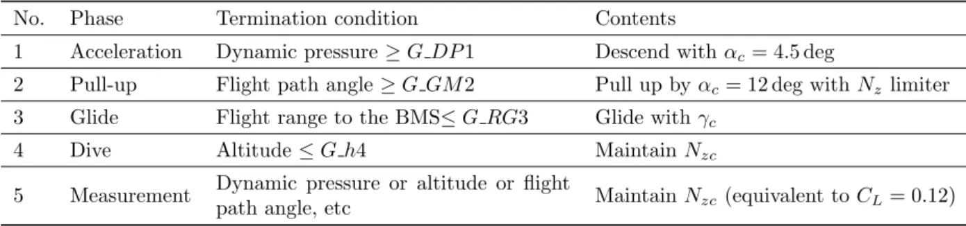
Table 2 Flight phases.
No. Phase Termination condition Contents
1 Acceleration Dynamic pressure≥G DP1 Descend withαc= 4.5 deg
2 Pull-up Flight path angle ≥G GM2 Pull up by αc= 12 deg withNz limiter
3 Glide Flight range to the BMS≤G RG3 Glide withγc
4 Dive Altitude ≤G h4 MaintainNzc
5 Measurement Dynamic pressure or altitude or flight
path angle, etc MaintainNzc (equivalent toCL= 0.12)
attitude controller. The second logic outputs the guidance commands based on a real-time trajectory prediction.
Summaries of the reference trajectories were presented in Ref. 5), 6). The flight experiment vehicle is lifted to
the altitude of 30 km by a stratospheric balloon. Then it is released with velocity of 0 m/s and a flight path angle
of -90 deg. The vehicle must fly with a Mach number of 1.3 and withCLof 0.12 over the BMS. The most desirable
flight condition at the BMS is designated as the target flight condition in this paper. Details of the target flight
condition are presented in Ref. 5), 6). The specific conditions are altitude of 7.67 km, Mach number of 1.3,
and flight path angle of -45.8 deg. The flight trajectory from separation to the target flight condition is divided
into five phases: acceleration, pull-up, glide, dive, and measurement (Table 2). The vehicle must consume the
position energy at the separation properly until reaching the BMS. Therefore, minimum and maximum flight
range trajectories exist. For the minimum flight range trajectory, the vehicle must consume its surplus initial
potential energy until reaching the BMS. For the maximum flight range trajectory, the initial potential energy
is equal to the energy necessary for flying to the BMS. An optimal problem is finally composed as follows: the
initial conditions are the separation conditions; the final constraints are the target flight conditions, and the
performance index is the flight range. Thus, reference trajectory data are calculated from optimization process
for various initial conditions. The guidance commands based on the reference trajectory data are outputted in
all phases except for dive phase.
The guidance law based on the real-time trajectory prediction is used in the dive phase to compensate for
the model errors and the uncertainties related to the actual flight conditions.
Details of the guidance law are presented hereinafter.
2
.2
Acceleration Phase
The vehicle accelerates with a constant angle of attack command of 4.5 deg, which is the same setting as in
the optimal problem.
A guidance law parameter of G DP1 is calculated once at the separation, and the flight phase goes to
the next phase when the dynamic pressure exceeds G DP1. From the obtained trajectory data, G DP1 is
formulated as a function of the flight range as is shown in Fig. 3.
2.3
Pull-up Phase
The guidance law outputs the constant angle of attack command of 12.0 deg, which is also the same setting
as the optimal problem. The angle of attack command is overwritten by the limiter to prevent the vehicle from
exceeding the load factor limit if the load factor reaches 3.5 G. Details of the limiter logic are presented in Ref.
0 1000 2000 3000 4000 5000 6000 7000 8000 -8 -7 -6 -5 -4 -3 -2 -1 0
16 18 20 22 24 26 28 30 Trajectory Data (G_DP1)
Trajectory Data (G_GM2)
G_DP1 = 13471 - 453.89*Range (km)
G_GM2 = 8.0777 - 0.52172*Range (km)
D yna m ic P re ss ure (P
a) Flight
P at h A ngl e (de gre e)
Flight Range (km)
Fig. 3G DP1 andGGM2. Both are defined by polynomials of the flight range.
When the flight path angle reachesG GM2, the flight phase changes. Figure 3 also showsG GM2 which is
formulated as similar toG DP1.
2
.
4
Glide Phase
The guidance law outputs a flight path angle command, which is formulated as three parts of polynomial
expressions of kinematic energy as shown in Fig. 4. The flight path angle command is made for typical flight
ranges. Figure 4 shows the maximum flight range case.
The glide phase is ended when the range-to-go reaches G RG3, which is a function of the altitude of
separation. This parameter is calculated by linear interpolation using the parameter values in Table 3.
2.5
Dive Phase
Although the guidance law outputs the commands based on the obtained trajectory data during the previous
flight phases, it must compensate for the model errors and the uncertainties related to the actual flight conditions.
Table 3G RG3 andG RG4.
Altitude (km) G RG3 (km) G RG4 (km)
26 5.679 3.860
27 5.660 3.824
28 5.815 3.986
29 6.153 4.322
30 5.958 4.130
-100 -80 -60 -40 -20 0
180 200 220 240 260 280 300
γc = 531.97 - 0.0021054×Energy (First part)
γc = 244.3 - 0.0011014×Energy (Second part)
γc = -59.168 + 0.00026209×Energy (Third part)
F
li
ght
P
at
h A
ngl
e (de
gre
e)
Kinematic Energy (kJ)
Black line means original data
Fig. 4 Gamma command is defined by a series of polynomials of kinematic energy.
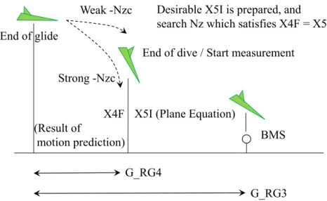
The guidance law based on the real-time trajectory prediction method serves this role.
Real-time trajectory prediction performed at the first cycle of this phase determines the load factor command
(G Nz4) and the final altitude of this phase (Gh4). When the altitude becomes less thanGh4 the dive phase is finished.
Figure 5 presents the concept of the method. On the one hand, the motion prediction function calculates
the final flight conditions of the dive phase(X4F) by integrating the equations of motion from the present flight
conditions to the flight range ofG RG4 with a constant load factor ofNzc. On the other hand,X5Iexpresses a
set of initial conditions of the measurement phase that satisfy the measurement conditions of Table 1 when the
vehicle flies withCLof 0.12 from these initial conditions to a BMS andX5Iis expressed using a plane equation.
Therefore, if X4F calculated using a certain load factor command satisfies X5I, the vehicle will satisfy the
measurement conditions naturally. Then the vehicle flies with the load factor during the dive phase and glides
withCL of 0.12 during the measurement phase.
Firstly, the contents of the motion prediction are described. During the dive phase, the attitude controller
maintains the bank angle of 0 deg in order to avoid interaction between the lateral motion and the longitudinal
motion and to prepare for the sonic boom measurement. Therefore, the motion prediction is performed only
for longitudinal motion. The independent variable is the flight range instead of time. Two reasons exist for this
formulation. If the flight range is selected as the independent variable, then theX4F that is the integrated
value from the present flight condition to the flight range ofGRG4 is obtained exactly. The other reason is to
reduce the computational cost by eliminating one variable of time. The state vectors are altitude, velocity, flight
path angle, and angle of attack. The control variable is the angle of attack command, and the independent
variable is the flight range. The equations of motion are as follows;
dh
G_RG4
G_RG3
End of dive / Start measurement
End of glide
X5I (Plane Equation)
X4F
(Result of
motion prediction)
Desirable X5I is prepared, and
search Nz which satisfies X4F = X5I
BMS
Weak -Nzc
Strong -Nzc
Fig.5 Concept of real-time trajectory prediction method.
dV
dR =
−D/m−gsinγ
V cosγ (2)
dγ
dR =
L/(mV) + (V /r−g/V) cosγ
Vcosγ (3)
dα
dR =
αc−α
TsVcosγ
. (4)
The angle of attack is modeled as controlled by the angle of attack command5, 6). This equation of angle of
attack response is formulated using a first-order delay model with a time delay based on the attitude controller
performance. Then the time constantTsis 1.28 s; the time delay is 0.6 s.
The final state of the dive phase, X4F, is obtained by integrating from the present condition to the flight
range ofG RG4.
Secondly, the approach of formulating of theX5I plane is described. The following initial conditions at the
beginning of measurement phase are presumed: the altitude is 8–14 km; the velocity is 300–460 m/s, and the
flight path angle is -90 deg to 0 deg. These ranges are set sufficiently wide based on the previous investigation.
Their intervals are, respectively 100 m, 1 m/s, and 1 deg. The angle of attack is the same value of the angle of
attack command and it is 4.2598 deg, corresponding toCLof 0.12 at Mach number of 1.3 in all cases. The flight
simulations are conducted for all combinations of the initial conditions, and the area where measurement of
the sonic boom is acceptable was investigated. The combinations of initial conditions are then selected so that
the desirable sonic boom reaching the area has a width of±2 km from the BMS. The plane equation ofX5Iis
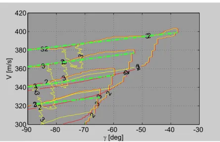
formulated as including those combinations of initial conditions. Figure 6 shows a sample figure ofX5Iplane.
Each pair of red and yellow solid lines in Fig. 6 show the contour lines of the desired sonic boom propagation
area for an initial altitude case. Red solid lines show the contours for the desired sonic boom propagates 2 km.
The yellow lines show those for 3 km. The green dotted lines show the approximated linear lines of contours
-90 -80 -70 -60 -50 -40 -30 300 320 340 360 380 400 420 2 2 2 2 3 3 3 3 3 2 2 2
3 3 3
3 2 2 3 3 3 2 2 3 3
[deg]
V
[m/
s]
Fig.6 Example of X5I plane.
expressed as;
2.4301×10⁻²h
−5.0245×10⁻⁴γ+ 1.8443
×10−3V = 1. (5)
Finally, the real-time trajectory prediction method is applied as shown below, where the guidance parameter
G RG4 is calculated by linear interpolation using the parameter values in Table 3.
Step 1) An initial value ofG N z4 is set from 0 G to−4.0 G every 0.1 G.
Step 2) The final state, X4F, is calculated by integrating the equations of motion from the present states to the
flight range ofG RG4 with givenG N z4.
Step 3) The points of intersection betweenX4F andX5I are calculated.
Step 4) Go to Step 1) and changeG N z4. IfG N z4 reaches−4.0 G, then go to Step 5).
Step 5) If several intersection points exist, thenG N z4 such thatγofX4F is the nearest to the target flight path
angle (=−60 deg) is selected. If there is no intersection, a minimum distance between X4F and X5I
plane case is selected.
2
.
6
Measurement Phase
The guidance law outputs Nzc to establish target CL, where Nzc is calculated using dynamic pressure
measured by an air data sensor and corresponds toCL of 0.12.
3
Evaluation of Performance
3.1
Presumed Conditions
Evaluation of the guidance law is performed by the simulations of motion of 3 degrees of freedom and by
supporting the vehicle as a point of mass. The only control variable is the angle of attack command. The states
are altitude, velocity, the flight path angle, the heading angle, latitude, longitude, and the angle of attack. This
Table 4 Model errors and uncertainties.
Item Value∗1 Distribution
Separation altitude 28–30 km uniform
Separation pitch angle −88.6±2 deg normal
CL Depends on Mach number normal
CD Depends on Mach number normal
Atmosphere Depends on altitude normal
Steady wind Depends on altitude normal
Ts ±10% normal
Separation position Inside of permitted separation area and desirable
separation area∗2 uniform
∗1
: The value indicates ±3σ value for a normal distribution and maximum/minimum
values for a uniform distribution.
∗2
: See Fig. 7 and Fig. 10
is controlled by adjusting the direction of its vertical fin to the BMS during the acceleration phase. If this
maneuver is controlled well, then the vehicle can fly straight to the BMS after pulling up. The control logic of
the direction of the vehicle’s fin is designated as an initial roll control. Although this control logic uses Euler
angles, the Euler angles cannot be defined in a 3 degree of freedom simulation. Therefore, this study does not
examine lateral guidance and presumes that the initial roll control is performed well. Details of the initial roll
control are described in Ref. 7).
Although steady winds are assumed for the flight simulation, the bank angle command is constantly set as
0 deg. Aerodynamic coefficients are modeled as a trimmedCLandCD6). Judgment for the requirements shown
in Table 1 is evaluated using ray path analysis8).
3.
2
Error Models
Error models and its related values are presented in Table 4.
3.3
Monte Carlo Simulation (MCS)
The distribution of separation points is portrayed in Fig. 7. Its vertical axis and horizontal axis respectively
represent south-north and east-west. Wherever the vehicle is separated from the area defined in Table 4, it selects
one of BMS and must generate a desired sonic boom above the BMS. ’Desirable separation area’ in Table 4 is
defined as follows; The vehicle can fly a certain range of distance which is determined by the separation altitude,
as is shown in section 2.1. Therefore, if the separation altitude is given, the minimum and maximum distance
of this achievable range of distance can be obtained. The intermediate distance of concentric circle with this
minimum and maximum distance from each BMS is ’Desirable separation area’.
With random combinations of errors shown in Table 4, 1 000 flight simulation cases were conducted. Results
of the flight simulations were checked first for whether they satisfy the constraints. If it exceeds the limitation
of dynamic pressure or the load factor, then it is categorized as a ‘violation’. If it satisfies all constraints, it is
evaluated then whether the measured sonic boom at the BMS satisfies the requirements presented in Table 1.
The result is classified as a ‘mission failure’ if the sonic boom does not satisfy all requirements. It is a ‘success’
-60 -40 -20 0 20 40 60
-60 -40 -20 0 20 40 60
Separation points Zone B BMS
Permitted separation area
X
(km
)
Y (km)
Fig.7 Distribution of separation points in MC.
-3 -2 -1 0 1 2 3 4
1.15 1.2 1.25 1.3 1.35 1.4 1.45
CD error
Steady wind error
S
uppos
ed e
rror (s
igm
a va
lue
)
Mach number at generating sonic boom Requested accuracy for Mach number
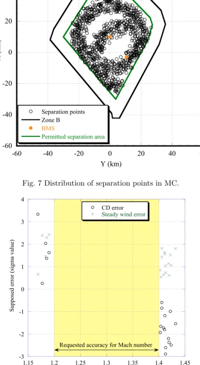
Fig. 8 Measured Mach number of mission failure case.
The mission failure cases are 19 cases. All mission failure cases violated the Mach number requirement. No
boom focusing case occurred. The success rate requirement to the guidance and control system is 90 %. This
success rate for the guidance law was accepted, because there are no device to control vehicle’s velocity.
-3 -2 -1 0 1 2 3 4
-3 -2 -1 0 1 2 3 4
S
uppos
ed s
te
ady w
ind e
rror (s
igm
a va
lue
)
Supposed CD error (sigma value)
Fig.9 Set values of steady wind and CD.
typically presumed error values of the mission failure cases. It shows a trend by which the Mach number is
below the requirement in case of a positiveCD error, and the Mach number exceeds the requirement in case of a negativeCD error. Figure 9 depicts CD error and steady wind error of the mission failure cases. It shows a trend by which the steady wind error becomes large in case of a small absolute value ofCD error.
Figure 10 shows separation points of mission failure cases. Although they show a weak trend by which failure
cases concentrate around the longer range and higher altitude, they spread widely in the desired separation area.
4
Result of Actual Flight
The flight experiment was conducted on July 24, 2015. Evaluations by actual flight results are presented
herein.
During flight campaign in 2014, there were no suitable day for flight test. After this campaign, separation
condition was expanded after precise investigation. As a results, the upper bound of desirable separation area
was extended from 30 km, as shown in Fig. 10, to 33 km, as shown in Fig. 11.
4.1
Actual Flight Trajectory
The vehicle was released within an extended separation area (Fig. 11), and it flew straightly towards a
selected BMS (Fig. 12). Figure 13 shows the actual flight trajectory with Mach number and an altitude. The
actual flight trajectory is accompanied with a predicted trajectory with no error and a simulated trajectory with
CDhaving -3σerror. In these trajectories, the initial altitude is the output of EGI (Embedded GPS/INS), and Mach number is that of ADS (Air Data Sensor). The simulated trajectory shows good correspondence with the
27.5 28.0 28.5 29.0 29.5 30.0 30.5
12 14 16 18 20 22 24 26
Separation position
Desirable separation area
S epa ra ti on a lt it ude ( km )
Target flight range at the separation (km)
Fig. 10 Separation positions of mission failure cases.
10 15 20 25 30 35
27 28 29 30 31 32 33 34 Al tit ud e [km] Range [km] Extended Separation Area Original Separation Area Separation Point
Fig. 11 Actual separation point.
shown in Fig. 14. As Fig. 14 showsCD has a large error, and this error was almost equivalent to -3σvalue.
4
.
2
Conputational Load on On-board Flight Computer
The CPU of the on-board flight computer is Power PC, MPC7410, and its clock frequency is 400 MHz. The
guidance law task was a 10 Hz cycle. All calculations were performed within the cycle.
4.3
Acceptance for Required Conditions
The maximum dynamic pressure was 57.26 kPa. The respective maximum and minimum load factors were
+3.72 G and -3.89 G.
Flight conditions of the measured target sonic boom were estimated as a Mach number of 1.386, change rate
of Mach number within±0.005 s−1, and CL of 0.122.
Therefore, the guidance law satisfied all the requirements.
27.5 28.0 28.5 29.0 29.5 30.0 30.5
12 14 16 18 20 22 24 26
Separation position
Desirable separation area
S epa ra ti on a lt it ude ( km )
-80 -60 -40 -20 0 20 40 -60
-40 -20 0 20 40 60
Y (km)
X
(km)
Zone B
Permitted separation area BMS
flight path separation point flight termination
Fig. 12 Flight path in horizontal plain.
Fig. 13 Actual flight trajectory.
4.4
R
e
sults of Real-Time Trajectory Prediction Method
The actual value of guidance parameters are aummerized in Table 5. The flight phase proceeded properly
from the dive phase to the measurement phase at the altitude ofGh4.
0 20 40 60 80 100 120 140 0
0.05 0.1
C D
time [s]
Estimated CD CD Model
Error Model( 3 )
Fig. 14 Estimated drag coefficient.
Table 5 Guidance parameters used in the actual flight.
Item Value
G DP1 2 408.9 Pa G GM2 -4.26 deg
G RG3 5 954.9 m
G h4 10 875.9 m
G N4 -2.9 G
G RG4 4 126.4 m
experiments must be the most difficult condition for the vehicle which has no effector for velocity control.
Nevertheless, the guidance law worked extremely well, leading to complete success.
From the viewpoint of managing risks, although CD is a parameter sensitive to the mission success, CD
estimated from the actual flight data was significantly differenet from model value. This implies that the
simulation model including error models was not as accurate as expected, and margin to mission success was
not satisfactory.
5
C
onclusions
This paper reported the guidance law of D–SEND#2. The guidance law used some trajectory data to realize
a desirable trajectory for an actual flight. Furthermore, the real-time trajectory prediction method was devised
to achieve all mission requirements against mathematical model errors and uncertainties.
The guidance law was evaluated using MCS, and the result was the success rate of 98.1%. Results clarified
that the guidance law has a little tolerance to the uncertainty of steady wind and of the model error of CD
because the vehicle has no engine or devices for velocity control.
Results of evaluation for guidance law using actual flight data show that the real-time trajectory prediction
estimated to be close to the presupposed minimum value, the guidance law realized a successful flight in which
all mission requirements are satisfied. On the other hand, this results direclty require that future works should
include enhancing the model building accuracy.
References
1) Honda, M. and Yoshida, K., D–SEND Project, Aeronautical and Space Sciences JAPAN, No.60 (2012), pp.
245-249 (in Japanese).
2) Kawakami, H., Shindo, S. and Naka, Y., Development and Operation of Sonic Boom Measurement System
in D–SEND#1, Aeronautical and Space Sciences JAPAN, No.61 (2013), pp. 1-7 (in Japanese).
3) Yanagihara, M. et al., Results of High Speed Flight Demonstration Phase II, Proceedings of the 55th
International Astronautical Congress, IAC-04-V.6.03, Vancouver, Oct. 2004.
4) Matteis, P. et al., The Italian Unmanned Space Vehicle FTB-1 Back to Fly, Experimental Objectives
and Results of the DTFT-2 Mission, Proceedings of the 61th International Astronautical Congress,
IAC-10.D2.6.7, Prague, Sep. 2010.
5) Suzuki, H. and Tomita, H., Optimal Trajectory Design for D–SEND#2 Vehicle, Proceedings of the 14th
Australian International Aerospace Congress, Melbourne, Feb. 2011.
6) Suzuki, H., Trajectory Design of D–SEND#2, JAXA Research and Development Report, JAXA-RR-15-002,
2015 (in Japanese).
7) Ninomiya, T., Suzuki, H. and Kawaguchi, J., Controller Design for D–SEND#2, Proceedings of the 3rd
CEAS Euro GNC conference, Toulouse, April. 2015.
8) TAKAGI, S., SUZUKI, S., and YOSHIKAWA, A., Ascent Trajectory Optimization Considering the Sonic
Boom, Journal of the Japan Society for Aeronautical and Space Sciences, No.48 (2000), pp405–410 (in
7-44-1 Jindaiji-higashimachi, Chofu-shi, Tokyo 182-8522 Japan URL: http://www.jaxa.jp/
Date of Issue: February 22, 2018 Produced by: Matsueda Printing Inc.