Multiple Steady States, Poverty Traps and Indeterminacy in the Uzawa–Lucas Model with Small and Large Educational Externality

Multiple Steady States, Poverty Traps and Indeterminacy in the Uzawa–Lucas Model with Small and Large Educational Externality

Shiro Kuwahara^†‡

University of Hyogo December 25, 2015

Abstract

This study attempts to comprehensively explain economic growth and stagnation in advanced and developing countries by endogenizing educational efficiency, the critical exogenous parameter in the Uzawa- Lucas model. In particular, we examine the dynamic properties of educational efficiency given its substantial role in yielding a long-run growth rate. The model yields multiple steady states under an in- tertemporal substitution elasticity that is greater than 1. The results reveal that a steady state with a higher growth rate shows indeter- minacy, and the identification of the steady states depends on how expectations are formulated. Thus, realizing long-run growth with a higher growth rate can be difficult owing to expectation formulations.

Keywords: Uzawa–Lucas model; Educational Externality; Multiple Steady States; Indeterminacy.

∗This work was conducted with financial support from JSPS KAKENHI Grant Number 15K03360 and the grant from Kobe Academic Park Association for the Promotion of Inter- University Research and Exchange.

†E-mail address: [email protected]

‡The author especially thanks the RoMacs participants at Kobe University for their insightful comments.

1 Introduction

This study attempts to develop a simple extension of the Uzawa-Lucas model (Uzawa 1965, Lucas 1988) and to provide an explanation for positive growth, no growth, and the multiplicity of economic paths. Economic growth theory focuses on realizing long-term growth and considers human capital as one of the key inputs for such growth. Given its simplicity and convenience, the Uzawa-Lucas model has been analyzed by introducing certain externalities;

for example, Mulligan and Sala-i-Martin (1993), Benhabib and Rerli (1994), Xie (1994), and Gomez (2003, 2004). Although these externalities are typ- ically introduced in the goods production sector, this study introduces the externality in the human capital accumulation sector. This setup yields not only an endogenously determined long-run growth factor but also a mul- tiplicity of economic paths, which would explain the diversity of economic paths that are described, for example, as the ”mystery of economic growth”

in Lucas (1988), which is a seminal paper on endogenous growth theory.

Furthermore, the present analysis of the multiplicity of economic paths also sheds light on stagnations caused by large economic shocks and the economic booms that precede the shocks. Of course, these phenomena are understood as monetary ones, (see, for example, Kindeleberger (1978)); how- ever, in the preceding expansionary term, we can observe TFP (total factor productivity) growth (see, for example, Kunieda and Shibata (2012)). The present study aims to replicate multiple economic paths, such as one with a high growth-rate path with the property of local indeterminacy and one with a low- or no-growth rate path with saddle point stability.

In the Uzawa–Lucas model, the exogenously given efficiency parameter of human capital accumulation (i.e., the educational efficiency parameter), and the linearity of human capital investment are critical determinants of the long-run growth rate. By denoting the educational efficiency parameter byb, the subjective discount parameter by ρ, and the intertemporal substitution elasticity by 1/θ, we obtain the long-run growth rate as (1/θ)(b−ρ). Further- more, if b > ρ, then this long-run growth is realized, and if b < ρ, no human capital accumulation is experienced and the economy is stuck in a no-growth trap. Thus, the realization of long-run growth is contingent on exogenously given parameter restrictions in the normal Uzawa–Lucas model.¹

By contrast, the present model assumes that the educational efficiency parameter bis endogenously determined but the dynamics are exogenous for economic agents. Therefore, we call this inserted mechanism, “educational

1In this case, Kuwahara (2013) is an exception, where an exogenousb is assumed, but long-run growth both with and without human capital investment is generated from an international knowledge spillover.

externality,” and extend the Uzawa–Lucas framework by introducing the dy- namics of educational externality efficiency. For simplification, we consider educational efficiency as a function of the economic production level cap- tured by physical capital endowment per human capital accumulation. As is broadly recognized, education is an engine for economic development, which implies that economic accumulation is generally accompanied by the educa- tional system. Thus, it is natural for a household to regard the educational environment as given rather than a private decision. Therefore, we can say that we develop a Uzawa–Lucas model with the minimum and simplest rela- tionship between educational efficiency level and economic growth to present the interrelationship between the two.

The results are summarized as follows. Too large educational external- ity makes economy explosive. The model contains multiple steady states with intertemporal substitution elasticity over 1², and there is a no-growth steady state in the case of lower educational efficiency and a higher subjective discount rate. The selection between the two depends on expectation forma- tion, although the steady state with a high growth rate shows indeterminacy properties under a small externality. Thus, it can be considered that the former corresponds to advanced economies because of more efficient educa- tion and long-run positive growth, while the latter to developing economies given the less efficient education level and absence of a growth steady state.

Therefore, the difficulties of maintaining high growth for advanced economies and achieving positive growth or initiating the growth path for developing economies are caused by expectation formation under indeterminacy.

This paper is organized as follows. Section 2 presents the model. Section 3 derives the steady states. Section 4 discusses the dynamics and stability of the system. Section 5 provides concluding remarks.

2 Model

2.1 Model with externality on educational efficiency

We assume a normal Uzawa–Lucas-type final goods production structure. It is constructed using physical capital (per capita capital stock is denoted by k) and human capital (per capita human capital stock ish) and is consumed as consumption goods (per capita consumption isc) and invested by physical capital (increment of per capita capital stock is ˙k); the final goods market

2Note that intertemporal substitution elasticity larger than 1 is necessary to generate multiplicity in the present study to generate multiplicity and this condition is supported by some empirical studies, for example, Vissing-Jorgenson and Attanasio (2003).

is competitive. The division rate of human capital in goods production is denoted as u(∈(0,1]); therefore, that of human capital in education is 1−u.

The clearing condition of the final goods market provides the dynamic equation of k as follows:

k(t) =˙ Ak(t)^α(u(t)h(t))^1−α

| {z }

y(t)

−c(t), 0< α <1, (1)

where A(>0) is the efficiency parameter of final goods production.

Human capital is assumed to be accumulated through the following equa- tion:

h(t) =˙ b(t)(1−u(t))h(t), b >0, (2) where b(t) is an efficiency parameter of human capital assumed to be a vari- able and the dynamics are introduced later in the paper. Furthermore, we assume that the household regards the dynamics as exogenously determined.

The representative household is assumed to have the following dynamical objective function on utility maximization:

max Z _∞

0

c(t)^1−θ−1

1−θ e^−ρtdt, (3)

wherec,θ(>0), and ρ >0 are per capita consumption, the constant relative risk aversion (CRRA) parameter, and subjective discount rate, respectively.

Note that the CRRA parameter corresponds to the reciprocal of intertempo- ral substitution elasticity in this class of utility functions.

Considering the dynamics ofb(t) as exogenous, the household maximizes this subject to the budget constraint, and the optimal conditions in the case of positive human capital investment, we call the ”Uzawa regime,” are calculated as follows:

λ(t) =c(t)^−θ, (4)

λ(t)(1−α)y(t)

u(t) =µ(t)b(t)h(t), (5)

ρλ(t)−λ(t) =˙ ∂H

∂k(t) =λ(t)αy(t)

k(t), (6)

ρµ(t)−µ(t) =˙ ∂H

∂h(t) =λ(t)(1−α)y(t)

h(t) +µ(t)b(t)(1−u(t)), (7)

t→∞lim e^−ρtλ(t)k(t) = 0, and lim

t→∞e^−ρtµ(t)h(t) = 0, (8) where λ and µ are the shadow prices of physical and human capital.

Then, we derive the dynamical equations in the Uzawa regime. Using (4), (5), (6), and (7), we derive the following equations:

ρ− λ(t)˙

λ(t) =αy(t) k(t)

¡:=r(t)¢

, (9)

ρ− µ(t)˙

µ(t) = λ(t)

µ(t)(1−α)y(t)

h(t)+b(t)(1−u(t)) =b(t), (10) Eqs.(6) and (7), and therefore, Eqs.(9) and (10), respectively, denote the optimal conditions for physical and human capital. r and b represent the marginal rate of transformation of physical and human capital, and as shown later, the growth rates of λ and µ and values of r and b are equated in the steady states with positive human capital accumulation.

Combining (4) and (9) yields the following Euler equation:

˙ c(t) c(t) = 1

θ

©αAx(t)^α−1u(t)^1−α−ρª

= 1

θ(r(t)−ρ), (11) where x:=k/h. Using (5), (9), and (10), we get

˙ u(t) u(t) = 1

α

"

b(t)−r(t) +αx(t)˙

x(t) − b(t)˙ b(t)

#

. (12)

Here, we introduce an assumption regarding the dynamics of b. For ed- ucational externality, we assume that the human capital endowment has a positive spillover on educational productivity, and thus, ^∂b_∂h > 0. Next, we need the property in which the effects are stationary in the steady states, and thus, additionally assume that the larger the economy, the smaller the spillover. We also assume the scale of an economy is captured by the per capita capital stock k, and thus, _∂k^∂b <0. Therefore, b is assumed as follows:

Assumption The dynamics of b negatively depends on x=k/h:

b(t) =b¡ x(t)¢

, b⁰(·)<0.

Furthermore, we assume that the elasticity ofb onx, denoted by ε(>0), is constant: ε := −^b0_b(x)^(x)x = (const). Thus, we specify the form of b(x) as follows: b(x) = ¯bx(t)^−ε, where ¯b(>0) is the total efficiency of human capital accumulation and elasticityεcaptures the externality intensity ofk andh. A larger ε means larger externality of human capital accumulation. Note that the assumption ε = 0 makes the present model the normal Uzawa–Lucas model.

3 Steady states

First, we consider the steady state with positive human capital accumulation, or the inner solution case, u^∗ ∈(0,1). We call this case the “Uzawa regime.”

A balanced growth path in the Uzawa regime is the state in which k, h, and c grow at a constant rate. In addition, u is constant and u ∈ (0,1), and therefore, x,q, andu are constant. We analyze the properties of steady states using three variable sets {x^∗, q^∗, u^∗}, where the index ∗ denotes the value at the steady state.

(1) and (2) imply that g_y^∗ =g_k^∗ =g_c^∗ =g_h^∗ =b(x^∗)(1−u^∗)¡ :=g^∗¢

and (4) and (5) imply −θg_c^∗ = g_µ^∗ = g_λ^∗. Therefore, by substituting g^∗ = −(1/θ)g^∗_µ into (10), we get

(1−u^∗)b(x^∗)θ =b(x^∗)−ρ. (13) This relationship provides two equations: one is an equilibrium relationship between x and u and the other is the equilibrium growth rate. The former can be immediately transformed from (13) and is given as

u^∗ = 1− 1

θ + ρ

θb(x^∗)(:= Ψ(x^∗)). (14) Imposing the condition in a steady state ( ˙x= 0 and ˙u= 0) on (12), we have

b(x^∗) = αAx^∗α−1u^∗1−α. (15)

Solving (15) with respect to u^∗, we obtain the following equation that shows the relationship between x and u in a steady state:

u^∗ =

µb(x^∗) α A

¶ ¹

1−α

x^∗(:= Φ(x^∗)). (16)

The intersection of the two equations, Ψ and Φ, determines the equilibrium value(s) of u^∗ and x^∗. Under the specification of b(x) = ¯bx^−ε, we have

u= Ψ(x) = θ−1

θ + ρ

θ¯bx^ε

| {z }

:= ¯Ψ(x)

, u= Φ(x) =

· ¯b α A

¸_1−α¹

x^1−1−αε ,

where ¯Ψ is the variable term of Ψ. These two functions have the following properties: Ψ is an increasing function and Φ(0) = 0, but the gradient of Φ depends on the externality level ε, and the sign of Ψ(0) depends on the reciprocal of the elasticity of the intertemporal substitution parameter θ.

Because the intersection of Φ and Ψ is so diverse, it is enormous and diffusive to observe all cases. Therefore, we make certain assumptions to confine the cases to an appropriate degree for the purpose of this study. To understand the shift from ε to Φ and Ψ, Fig. 1 is an ad referendum drawn under the assumption θ < 1, and 1− ¹_θ +_θρ^¯b > 0. ³ Note that if ε → 0, the model is reduced to the normal Uzawa–Lucas model, and ^θ−1_θ + _θρ^¯b > 0 is one of the necessary conditions for the inner solution.

Next, we check the steady state withnohuman capital investment; there- fore, there is no growth in the long run. We call this case the ”Solow regime,” where all human capital is employed in the final goods produc- tion sector; therefore, u(t) becomes constant u = 1. In this case, human capital investment is not optimal for a household, and the model resembles the Solow model. Substituting u = 1 into the Euler equation, we obtain r^∗∗ = αAx^∗∗α−1 = ρ, and therefore, x^∗∗ =

hαA ρ

i ¹

1−α, where ∗∗ denotes the steady state value of the Solow regime. The difference between the Solow model and Solow regime in this study is the existence of the non-profitable condition for human capital investment. This phenomenon emerges when the MRT of human capital is lower than that of physical capital; there- fore, we have the following condition: b(x^∗∗) < αAx^∗∗α−1(= ρ), that is,

¯b < ρ^1−1−αε (αA)^1−αε (:= ˜ρ). From this, we obtain the following Lemma:

Lemma 1-1

¯b

½ >

<

¾

˜

ρ ⇔Economy

½ does not have has

¾

the Steady State in the Solow Regime.

We might term a country with ¯b > ρ˜as ”advanced country” and one with

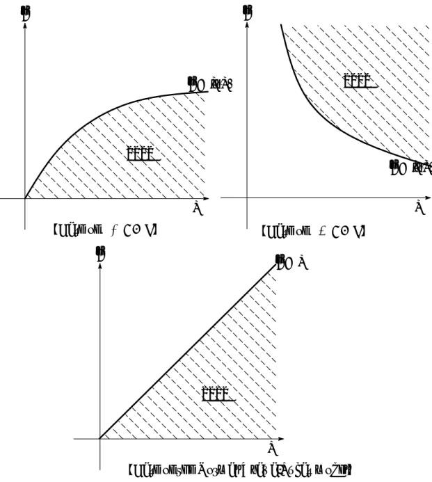
¯b < ρ˜ as ”developing country.” The domain that the Solow regime steady state exists is depicted on ¯b-ρ plain in Fig. 2. Similar to the normal Uzawa–

Lucas model, the educational efficiency parameter ¯b and subjective discount rate ρ determine the no-growth steady state. Under a more intense exter- nality, the upward-sloping relationship between the parameters is disturbed and a small subjective discount and high educational efficiency yield poverty traps. In addition, the production parameter also affects the condition of no-growth traps. Higher parameters of production A and physical capital α (higher α decreases human capital efficiency in production 1−α) make higher educational efficiency necessary for the existence of long-run positive growth; these affects relatively disadvantage education.

3In the iinterval ofε∈(0,1−α), Φ is always increasing.

To clear the relationship between the above condition and equations Ψ and Ψ, we define x = Φ⁻¹(u) and x = Ψ⁻¹(u) as the inverse function of u = Ψ(x) and u = Φ(x) and x_φ := Φ⁻¹(1) = {¯b/(αA)}^−1+α+ε1 and x_ψ :=

Ψ⁻¹(1) = (¯b/ρ)^1/ε. Then, we derive the following:

½ x_φ< x^∗∗< x_ψ xψ <(x^∗∗)< xφ

¾

⇐⇒¯b

½ <

>

¾

˜ ρ.

Next, we explore the steady state in the Uzawa regime. Here, we consider two cases: one with the Solow regime and the other without.

Case I: Small externality case (ε∈ (0,1−α)) At first, we inquire the case with small externality, specified as follows:⁴

0< ε <ε¯:= 1−α 2−α,

µ

¯ ε∈

µ 0,1

2

¶¶

.

. The phase of steady states with ¯b >ρ˜and ε∈(0,1−α) is depicted onρ-¯b plane in Fig.3 (a).

To obtain the condition of steady states, we reconsider the ralation be- tween Φ and Ψ from the viewpoint of u, thus we obtain the equation u = Ψ(Φ⁻¹(u)) which gives the euqilibrium, and this equation is transformed into

(L(u) :=)u+ 1−θ

θ = 1

θΩ^β+ε1 u^β+εε (:=R(u)),

where β := 1− ^ε_¯ε and Ω := ^ρ_¯b^˜. In the case discussed here, β > 0, Ω∈ (0,1) and _β+ε^ε ∈(0,1) respectively hold. We respectively define the LHS and RHS of the above equation as L(u) and R(u). The graph of L(u) and R(u) are given by Fig.4(a).

Lemma 1-2 Under the assumptionθ ∈(θ,1),¯b >ρ, and˜ ε∈(0,ε), namely¯ high intertemporal elasticity of substitution, high educational efficiency, and small educational externality, we always have multiple equilibria {E₁, E₂} where both equilibria are related with long-run positive growth.

4The properties of the intersection of Ψ and Φ are changed byε, the intense parameter of externality, and the properties are divided by some thresholds such as ¯εand 1−α(>ε).¯ For example, 1−α is the threshold that the incline of Φ is change from increasing to decreasing for the increment of ε. Then, the above assumption given in (R1) implies that we focus on the case with small externality. To understand the implication of ¯ε, we check the gradient of these two lines. We can derive ε from the following equation:

¯ ε = arg

n ε

¯¯

¯

³_¯

Ψ⁰(x)x Ψ(x)¯ =

´

ε= 1−_1−α^ε

³

= ^Φ_Φ(x)^0(x)x

´ o

. Therefore, the ¯ε is the point where Φ and Ψ has the same buckling, and ε >(<)¯ε implies that for small (large) externality, buckling of Φ is larger (smaller) than that of Ψ.

Proof) Since L(0) > R(0) and L(1) > R(1), which are respectively pro- vided by θ <1 and ¯b > ρ, the case, in which˜ L and R have two equilibrium u^∗₁ and u^∗₂, is conditioned byL(u)> R(u) for ∃u∈(0,1).

To show this, we define ˆu := arg©

u|R⁰(u) = 1(= L⁰(u))ª

, namaely ˆu is the point where the gradient ofR is equaled to unity which is the gradient of L, and L(ˆu)> R(ˆu) is to be proved. Since R⁰(ˆu) = 1 and R⁰(u) = _β+ε^{ε R(u)}_u , we have R(ˆu) = ^β+ε_ε u(:=ˆ Q(ˆu)). R(ˆu) = Q(ˆu) gives

ˆ u=

µ ε β+ε

¶^β+ε

β µ

1 θ

¶^β+ε

β

Ω^1β .

Substituting the ˆuderived here into the conditionL(ˆu)> R(ˆu), we obtain the condition ˆu > u, where u := _β^ε1−θ_θ . ˆu is the intersection of Q(u) and L(u). From the Fig.5(a), where ˆuanduare drawn on (1/θ)-uplane, we have ˆ

u > u for (1/θ) > 1, namely, θ < 1, thus, R(ˆu) > L(ˆu). Thus, we have u^∗₂ < u < u < uˆ ^∗₁.

From the necessary condition ˆu <1, we haveθ > θ, whereθ := _β+ε^ε Ω^β+ε1 (∈

(0,1)). (Q.E.D)

It should be noted that u^∗₂ < u < u < uˆ ^∗₁ also plays an important role in the determination of stability, which is discussed in the Ch.4 in this paper.

Here, we change the condition ¯b >ρ˜in the above lemma into ¯b < ρ, then˜ the equilibrium E₁ is vanished and E₀ alternatively emerges⁵. The phase of steady states are given in the Tab.1(b).

Case II: Middle externality Case (ε∈(¯ε,1−α)) Next, we inquire the case with middle externality. When we additionally adpot the assumptions;

θ > 1, and ¯b < ρ, we obtain the phase of steady states are depicted on˜ ρ-¯b plane in Fig.4 (b). In this case, we obtain the following lemma:

Lemma 1-3 Under the assumptionθ > 1,¯b <ρ, and˜ ε∈(¯ε,1−α), namely low intertemporal elasticity of substitution, low educational efficiency, and relatively large educational externality, we obtain multiple equilibria{E₀, E₁, E₂} where both equilibria {E₁, E₂} are related with long-run positive growth, and the equilibrium {E₀} is related with no growth traps.

5It should be noted thatE0 is always existing under ¯b <ρ.˜

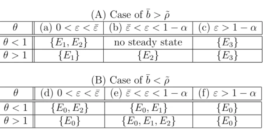
Table 1: Equilibrium Set (A) Case of ¯b >ρ˜

θ (a) 0< ε < ε¯ (b) ¯ε < ε <1−α (c) ε >1−α θ < 1 {E₁, E₂} no steady state {E₃}

θ > 1 {E1} {E2} {E3}

(B) Case of ¯b <ρ˜

θ (d) 0 < ε <ε¯ (e) ¯ε < ε <1−α (f) ε >1−α θ < 1 {E0, E2} {E0, E1} {E0} θ > 1 {E₀} {E₀, E₁, E₂} {E₀}

Proof) In this case, we obtain β < 1, Ω < 1, and _β+ε^ε >1. Since L(0) >

R(0) andL(1) > R(1) hold in this case, the property thatL andR have two equilibrium u^∗₁ and u^∗₂ is conditioned byL(u)> R(u) for∃u∈(0,1).

In Case II, we also obtain the same threshold value ˆu and ¯u, depicted in Fig. 5(b), where

³ ε β+ε

´^β+ε

β Ω^β1 > 1 is derived from _β+ε^ε > 1 and Ω^1β > 1.

Thus, we also obtain u^∗₂ < u < u < uˆ ^∗₁. (Q.E.D)

Here, we also change the condition ¯b <ρ˜in the above lemma into ¯b >ρ,˜ then the equilibria E0 and E1 are vanished. The phase of steady states are given in the Tab.1(a).

Case III: Large externality case (ε > 1−α) The last case is the one with large externality. In this case, the function Φ becomes decreasing, so multiple steady states does not emerge. The pattern of steady states is determined by only the condition ¯b > ρ˜ or ¯b < ρ. The obtained relsut is˜ given in Tab.1 in the colum of ε >1−α, and depicted in Fig. 3 (c) and (d).

E₃ denotes the equilibrium with positive human capital accumulation in the Case III.

Finally, we check the TVC. From (8), we haveρ≥γ_λ^∗+γ_k^∗ andρ≥γ_µ^∗+γ_h^∗, where γ_Z := ^Z_Z^˙. Since p = µ/λ and x = k/h are constant in steady states, both conditions are satisfied if one condition is shown to hold. Substituting γλ =−θγc =−θg^∗ = −(b^∗ −ρ) and g^∗_k =g^∗ =b^∗(1−u^∗) into ρ ≥ γ_λ^∗ +γ_k^∗ yields b^∗u^∗ ≥ 0, threfore, the steady states in the Uzawa regime obtained above always satisfy the TVC conditions.

Note that in the no-externality case, ε = 0, the condition becomes the same as that in the normal Uzawa–Lucas model. In the following section, we analyze the stability of the obtained steady states.

One of results obtained here is that an developing country migiht have more possibility for multiple steady states, which corresponds to the large flucuation of growth dynamics of those countries. Note that intertemporal substitution elasticity larger than 1 (CRRA parameter is smaller than 1) is supported by some empirical studies, for example, Vissing-Jorgenson and Attanasio (2003). Under this condition (θ < 1), advanced country with

¯

ε < ε < 1−α, lose steady state, and as is given in Appendix, E₃ is shown to be source around ε = 1. These results imply that too large externality diffuses economy, so hereafter, we confine our analysis mainly to the case 0< ε < ε.¯

4 Dynamical system and stability

Because the case without human capital accumulation (which is related to {E₀}) is reduced to the standard Ramsey model, saddle stability is easy to prove. Thus, we concentrate on the cases with positive long-run growth (related to E₁, E₂).

4.1 Dynamical equations

Let us define the following variables:

w(t) := (1−α)Ax(t)^1−αu(t)^1−α, and p(t) := µ(t)

λ(t). (17)

Note thatpcorresponds to the stock price of human capital if the agents can trade their ownership of human capital in the asset market.

From r (defined in (9)) and win (17), we obtain the following two prop- erties:

r(t)^1−αw(t)^α =α^1−α(1−α)^αA, and r(t)

w(t) = α 1−α

u(t)

x(t). (18) On the other hand, substituting r and win (18) yields

w(t)h(t) = b(t)p(t)h(t), namely w(t) = ˜p(t). (19) where ˜p:=b p, which represents the efficiency-adjusted stock price of human capital. Substituting (19) in (18), we have the interest rate as a function of

p as follows:

r(t) = r(˜p(t)) := ˜p(t)^−1−αα , for ∀t, and r⁰(·)<0. (20) where the property r⁰(·)<0 comes from the well-known Stolper–Samuelson theorem. From (18)–(20), we obtain

u(t) = 1−α α

r(˜p(t))

˜

p(t) x(t). (21)

Thus,u(t) is determined by ˜pandx. Next, we analyze the dynamical system using the variable set {˜p(t), q(t), x(t)}.

Defining the new variableq :=c/k, we rewrite the system constituted by (1), (2), (11), and (21) as follows:

˙ q(t) q(t) =

µ1 θ − 1

α

¶

r(˜p(t))− ρ

θ +q(t), (22)

˙ x(t) x(t) =

·1 α +υ¡

x(t),p(t)˜ ¢¸

r(˜p(t))−q(t)−b(x(t)). (23) where υ(x,p) :=˜ ^1−α_α ^b(x)x_p˜ . Note that u^∗ =υ^∗ holds in the steady states with positive human capital accumulation since r^∗ =b^∗ holds.

Using (9), (10) with the definition of ˜p(= b µ/λ), and specification of b(x)(= ¯bx^−ε), the dynamics of ˜p are given as

˙˜

p(t)

˜

p(t) = b(t)˙

b(t) +µ(t)˙

µ(t)− λ(t)˙

λ(t) =r(˜p(t))−b(x(t))−εx(t)˙ x(t),

=

½ 1−ε

·1

α +υ(x(t),p(t))˜

¸¾ r¡

˜ p(t)¢

+ε q(t)−(1−ε)b(x(t)). (24) The three dynamical equations, (22), (23), and (24), constitute the economic system of the model.

4.2 Stability analysis

In this section, we discuss the dynamics of the model. From Eqs. (22)–(24), we obtain the linearized dynamical equations {p,˙˜ q,˙ x}˙ as follows:



 p(t)˙˜

˙ q(t)

˙ x(t)



=J^∗



 p(t)˜ −p˜^∗ q(t)−q^∗ x(t)−x^∗



,

where J^∗ :=





u^∗ α x^∗

£−α+ε¡

1 + _1−α^αu∗¢¤

˜

p^∗ ε˜p^∗ (1−ε)^εb(x_x∗^∗)(1−u^∗)˜p^∗

¡1− ^α_θ¢ _u∗

α x^∗q^∗ q^∗ 0

−^u_α^∗¡

1 + _1−α^αu∗¢

−x^∗ b(x^∗)£

(1−ε)u^∗+ε¤



. The stability around the steady state depends on the sign of the eigenvalues derived from the above linearized system. To investigate the sign of the values, we define the following characteristic equation for the above system:

Γ(λ) = −λ³+T r^∗λ²+B^∗λ+Det^∗,

where λ, T r^∗, and Det^∗, respectively, denote the eigenvalue, trace, and de- terminant of this system. Then, B^∗ is derived as follows:

B^∗ =−u^∗

·

q^∗b^∗ + p˜^∗

x^∗ (q^∗−b^∗u^∗)

¸

| {z }

:= ¯B

+ε

·

2b^∗p˜^∗u^∗ αx^∗

µ

1 + α u^∗ 1−α

¶

− p˜^∗q^∗u^∗ α x^∗

³ 1− α

θ

´

+b^∗q^∗(1−u^∗)

¸ . From J^∗ and using q^∗ = ^r(˜_α^p∗)[1 + (1−α)^b(x)x_p˜∗^∗] +b(x^∗), we haveT r^∗ andDet^∗ as follows:

Det^∗ =b(x^∗)˜p^∗q^∗u^∗ x^∗

·

−©

(1−ε)u^∗+εª +ε

µ1

θ + u^∗ 1−α

¶¸

| {z }

:=Θ

T r^∗ =r(˜p^∗) α

·

(1−α) µ

1 + b(x^∗)

˜ p^∗

¶ +ε

µ

1 + αu^∗ 1−α

¶¸

+b(x^∗)©

(1−ε)u^∗+εª

>0.

Therefore, the sign of Θ affects the dynamical properties through the sign of the determinant.

Lemma 2-1 E₁ is saddle stable and E₂ is the source or indeterminacy.

Proof) From the Routh–Hurwitz theorem (see, for example, Benhabib and Perli (1994) and Arnold (2000)), Det^∗ < 0(> 0) and T r^∗ > 0 imply the set of eigenvalues {+ +−} ({+ + +} or{+− −}), and therefore, saddle stability (source or indeterminacy). Thus, the dynamical properties in the present case depend on the sign of Θ, which yields the condition

u^∗

½ >

<

¾ u⇔

½ saddle stable

source or indeterminacy . (25) Applyingu^∗₂ < u < u^∗₁, which is derived in the proof of Lemma 1-2 to (27), we have the result thatE₁is saddle stable andE₂ is the source or indeterminacy.

(Q.E.D)