Journal of Hydroscience and Hydraulic Engineering Vol. 20, No.2 November, 2002, 51-69
A SIMULATION STUDY OF AQUEOUS AND GAS PHASE DNAPL MIGRATION IN SHALLOW UNSATURATED LAND ELEMENTS
By
RABINDRA RAJ GIRl
Geosphere Research Institute, Saitama University, 255 Shimo-okubo, Saitama-shi, 338-8570, Japan, E-mail: [email protected]
KUNIAKI SATO
Geosphere Research Institute, Saitama University, 255 Shimo-okubo, Saitama-shi, 338-8570, Japan, E-mail: [email protected]
AKlRA WADA
Nihon University, CollegeofIndustrial Technology, 1-2-1, Izumi, Narashino, Chiba, Japan, E-mail: [email protected]
YASUHIDE TAKANO
Department of Civil Engineering, Kinki University, 3-4-1 Kowakae, Higashi-Osaka, Osaka 577-8502, Japan, E-mail: [email protected]
and TAKASHI SASAKI
Ark Information Systems, Inc., 4-2 Gobancho Chiyoda-ku, Tokyo, Japan, E-mail: [email protected]
SYNOPSIS
Knowledge of DNAPL migration behaviours in shallow unsaturated land elements might be useful in· characterizing and deciding suitable remediation techniques for DNAPL contaminated sites. One-dimensional simulations of simultaneous heat, moisture, and gas and aqueous phases DNAPL transport in soil due to diurnal land-atmosphere interactions was carried out The top a.ll-m soil was initially contaminated with uniform DNAPL concentrations in aqueous and gas phases. Two cases of moisture content scenario were presented in the simulations. The results indicated that vegetation cover played significant roles in soil heat and moisture budgets in addition to soil composition and their properties.
Vegetation cover significantly reduced the incoming solar radiation to the ground surface resulting to smaller diurnal fluctuations in soil temperature and moisture contents in vegetated lands. The decrease in aqueous phase DNAPL concentrations in the contaminated soil layer and the downward migration depths were relatively bigger in vegetated lands.
Rainfall percolation further reduced diurnal soil moisture fluctuations resulting to bigger aqueous phase DNAPL migration depths. Gas phase DNAPL exhibited bigger vertical spreading tendency. Further investigations including other process in the contaminant transport equations, and sensitivity analyses on their relative importance would provide more insight in the matter.
- 1 -
1. INTRODUCTION
Subsurface contamination by Dense Non-aqueous Phase liquids (DNAPLs) has more than half century's history in the industrialized countries. The production and use of some of the DNAPLs, such as trichloroethylene (TCE), were first reported in the United States, Germany and United Kingdom in the early ·1900. Their production and use increased proportionately with the industrial development. At a time, the use of dense chlorinated solvents was considered as an indicator of industrial and economic growth. A close look into the history of DNAPL production and use reveals that the major subsurface contamination OCCUlTed in between 1950 and 1980. From early 1980s onwards, a huge flux of subsurface contamination repOlts were available resulting to active engagement of governments, policy makers, scientists and researchers to prevent further contamination and remediate the contaminated sites.
DNAPL's peculiar physical properties render them highly mobile as well persistent in the subsurface environment. Bigger densities, lower viscosity and smaller interfacial tension with liquid water enhance rapid migration. Most of the DNAPLs are highly volatile resulting to increased gas phase contamination. Lower degradability and smaller absolute solubility with water keep them in the subsurface as DNAPL pool for longer period. On the other hand, appreciable relative solubility, for example TCE, contaminates soil and groundwater many folds higher than the maximum contaminant level (MCL) specified in the environmental standards.
Many literatures are available on DNAPL subsurface contamination and remediation.
Depending on subsurface moisture conditions, contamination cases can be broadly classified into two: (a) saturated and (b) unsaturated. Since the focus of this paper is on the second point, some of the relevant literatures on DNAPL subsurface contamination in unsaturated conditions are briefly discussed in this section. Sleep and Sykes (1989) carried out an extensive numerical analysis on TCE transport in variably saturated soils. Dissolution and volatilization of immobilized TCE mass transport in aqueous and gas phases and gas-liquid partitioning between aqueous and gas phases were taken into consideration for two different surface boundary conditions. The simulation results revealed that the consideration of gas- liquid partitioning between aqueous and gas phases resulted to greater horizontal and vertical spreading of aqueous phase plume. TeE dissolution rate increased and volatilization rate decreased by the inclusion of gas-liquid partitioning. The increase in mass transfer coefficients increased the gas and aqueous phase concentrations. More interestingly, the change in ground surface boundary conditions showed significant impact on lateral and vertical plume spreading in aqueous and gas phases. Impermeable boundary at surface enhanced such spreading of plumes.
Arands et a1. (1997) used modeling and experimental approach to study the gas phase diffusion of volatile organic contaminants (VOCs) in unsaturated soil. The results indicated that the volume fraction of vapor phase in soil significantly influenced diffusive transport of VOCs in unsaturated conditions. As soil water content increased, the vapor filled volume fraction in soil became more tortuous resulting to reduction in vapor phase transport. Conant et a1. (1996) calTied out similar field and numerical modeling investigation on TCE vapor transpOlt in unsaturated soil zone. The field experiments revealed that a vapor plume migrated several meters lateraJly and downward to the capillary fringe within only a few days.
Comparisons between the results for winter and. summer conditions indicated that seasonal
temperature variations could have a strong effect on source· concentrations, vapor transport
rate and contaminant mass transport. Variability in organic carbon content showed significant
control over the relative migration rates at different soil depths. Many authors mainly focused
on volatilization and gas phase VOC migration in the subsurface (e.g. Wilkins et aI., 1995).
Yates et aI. (2000) developed and compared several analytical solutions to simulate one- dimensional VOC gas transp0l1 in unsaturated layered soil system. The experimental investigation of Maraqa et aI. (1999) on the effect of water saturation on retardation of groundwater contaminants indicated that volatilization might have significant impact on retardation of organic compounds with higher values of Henry's constant in aquifer with low organic matter content.
In the recent past, some authors investigated the effects of vegetation on VOC and DNAPL migration in the subsurface. An experimental study of Zhang et al. (1998) reported that vegetation accelerated TCE upward movement due to root water uptake and plant transpiration. This process enhanced mass transfer and TCE dissolution resulting to increase in TCE concentration both in aqueous and gas phases. Narayanan et aI. (1996) used experimental and modeling approach to examine the fate of TCE in a chamber with alfalfa plants. The results indicated that the moisture distribution in soil significantly affected TCE transport in the subsurface. The major TCE loss in soil was through the volatilization mechanism. Root water uptake and evapotranspiration phenomena associated with the actively growing alfalfa plants enhanced upward moisture movement resulting to increased volatilization. However, very little is known about the impact of vegetation on the fate of DNAPLs and other chlorinated solvents in the subsurface and hence more specific studies are needed to reach to the realities.
The change in heat and moisture budget is one of the most important factors in assessing the fate of dense chlorinated solvents in the shallow subsurface. Industrialization has enhanced the widespread use of DNAPLs, where as urbanization significantly changed the existing heat and'moisture budgets in the topsoil. It is essentially important to understand the extent of contamination and local environmental situation before applying any remedial techniques to a DNAPL contaminated site.
Diurnal interactions between soil and atmosphere play vital role on the fate of volatile contaminants in shallow subsurface, and the degree of interaction varies with various surface and subsurface conditions. However, the fates and transport behaviors of these contaminants in shallow subsurface for different land-use conditions are not well investigated.
The objective of this paper is to compare aqueous and gas phase TCE (a typical DNAPL) migration into shallow subsurface from the top contaminated soil layer in four different land- use conditions. The four land elements, bare soil, short-grass covered land, forest covered land and porous pavement, are taken into account in this study, because they are typical surface coverings and land-use conditions. The knowledge of heat and mass budgets, including volatile contaminants, in these elements are expected to be of significant importance in land planning. Only the simplest aspect of vegetation is considered here to compare the fate of TCE in aqueous and gas phases. Two cases of vegetation are presented here (short grassland and densely forested land) to compare the impact of vegetation types.
Soil composition and its hydraulic and thermal properties characterize the land-use conditions in addition to the vegetation parameter.
2. SIMULATION MODEL AND TRANSPORT EQUATIONS 2.1 Simulation Model
Soil-Atmosphere Linking Simulation Algorithm (SALSA) coupled with equations for simultaneous transport of heat, moisture and DNAPL in soil has been used in this simulation.
ten Berge H.F.M (1990) first developed SALSA model to predict heat and moisture transfer between bare topsoil and lower atmosphere due to diurnal interaction between them. The accuracy of the model and the usefulness of the simulation results were evaluated in the earlier investigations (ten Berge, 1990 and Son et aI., 1999). Later, Sato et aI. (200 1)
- 3 -
attempted to use the model for four different land-use conditions. In this paper, we have attempted to modify the existing SALSA model by introducing a system of equations for simultaneous transpOlt of heat, moisture and dense volatile chlorinated solvent (DNAPL) in the subsurface and compare the migration behaviour in aqueous and gas phases among the four different land-use conditions. A conceptual diagram of land-atmosphere interaction with four types of land elements (land-use conditions) is presented in figure 1. The four land elements exhibited different surface and subsurface characteristics. The bare soil represents the land without any vegetation at the ground smface. The sholt-grass element denotes the land covered with sparse shOlt-grasses. The forest element represents densely forested area.
Similarly, the porous pavement element indicates compacted pavement materials that are intended for drainage or parking purposes in urban areas. Even though, all these four elements are shown together in figure I, they are dealt with separately in simulation studies while investigating the fate and transport behaviours of the contaminant under the conditions set for each element.
• ·.··fi
Rainfall
I ! ! I ' ! I
; I !
I'I I
l " .
I
vtvvvvv
DNAPL volatilization
+HH
" -~
.: .... j '
',~...
:.- -,.'If.'~· Grolc1ndwater table
liiiil:ii
Mixing ratio
( Pot.
Temp.
o
Fig. 1 Conceptual diagram for land-atmosphere interaction
2.2 Transports in the Atmosphere
A detailed description of the transport equations in the atmosphere is presented in ten Berge (1990) and other similar literatures. We have outlined only the main equations in this section.
Momentum, heat, moisture and turbulent kinetic energy (TKE) transport in vertical direction in the atmosphere are expressed by the following equations:
(1)
(2)
(5) (4)
where, u and v = wind velocities, 1: = momentum flux, B = air potential temperature, E =
water vapor flux density, H = sensible heat flux, f = coriolis parameter, q = moisture mixing ratio, Pa = air density, C p = specific heat of air at constant pressure, e = TKE, A.M = length scale, c = empirical parameter, T a = air temperature and K M = transport coefficient for momentum.
The following equations express the fluxes of momentum, sensible heat and water vapor near the ground surface:
{U(ZIII)-U(ZO)} {v(zm)-v(zo)}
Tx=Pa ;Ty=Pa
raM raM
H= C {Ta(zlII)-Ta(zo)}. E= {q(Zn,)-q(zo)}
Pa
p, P a )
r
aH(r
av+ r
cwhere, Zo = surface roughness height, Zm = height at which the state variables are measured, r a
= aerodynamic resistance and r c = vegetation resistance.
The subscripts M, H and V in equations (4) and (5) indicates momentum, heat and vapor respectively.
2.3 Transports in the Subsurface
_ Simultaneous transport of heat, moisture and DNAPL in aqueous and gas phases are . considered in the subsurface migration (Takano et aI., 200 I). Moisture transport in unsaturated soils is considered to be in liquid and vapor phases, which includes vaporization and condensation. The following equation expresses liquid water transport in the unsaturated soil.
a~~B.)~kg ~ {(p::"Ja~. H~)~ f~:'J~}+kg ~(P::" J (6)
- KG (8 - B,J(xwPvsal - p. )
where, (h. = volumetric liquid water content, k = saturated soil permeability, krA. = relative soil permeability, M = DNAPL molar mass, T s = soil temperature, R = universal gas constant, C
= aqueous phase concentration, f: = soil porosity, \jim = matric potential head, KG = coefficient of internal evaporation for water, P v = water vapor pressure, P vsat = saturated water vapor pressure and XW = mole fraction for liquid water.
Water vapor transport is governed by the following equation.
~{(8- B;.)Pv} = (~17Dalm.)~[(8 - B;. ,J ~(Pv J}] + K G R,.(8 - B;.XXwPvsa( - pv) (7)
at 1'., az 1. az T s .
where, ~ = correction factor for vaporizing area, 11 = tortuousity factor, D atmv = water vapor diffusivity in atmosphere and R v = gas constant for water vapor.
Two-phase DNAPL transport in the subsurface is taken into account in this simulation, which includes volatilization. The effect of immiscible phase on aqueous and gas phase transport is neglected. The aqueous phase DNAPL transport including adsorption on the solid matrix can be expressed by the following equation.
-5-
(8)
ac aB, a ( a c ) ( )
(B, +PdKd)-+C-=- B,Dc--V;C -Kv(c-B, ) H"C-C g
at at az az
+ CK G (c - ~ )(X".Pvsot - pv) PI
where, Pd = apparent density of soil, Kd= aqueous phase DNAPL adsorption coefficient, Dc = aqueous phase DNAPL diffusion coefficient, VA. = liquid water Darcy velocity, K y = DNAPL gas generation coefficient, H
y= dimensionless Henry's constant for DNAPL and C g = gas phase DNAPL concentration.
Diffusion and convection are the two important mechanisms taken into account in equation (8). The first and the second terms in the right hand side of the equation represent these two processes respectively. The third tenn accounts for the volatilization of the dissolved phase DNAPL. The last term does indicate aqueous phase concentration change due to liquid water vaporization, which is an important telm in contaminant transport (Takano et a1., 2001).
However, its relative significance in the case of DNAPL contaminants is yet to be investigated.
The following equation expresses gas phase DNAPL transport in the subsurface, which includes diffusion and adsorption on the solid matrix.
( c-B, +PdKd ---Cg-=TJ- Do1mg c-B, - - +Kv c-B, HvC-C . - ) aC at g a~ a t a z a { ( ) ac az g } ( ) (
g) (9) where, D atmg = DNAPL gas diffusion coefficient in the atmosphere and K
d= gas phase DNAPL adsorption coefficient.
Diffusion is assumed to be the dominant gas phase contaminant transport mechanism in the fine-grained unsaturated soil domain, and hence other transport processes, such as density-driven advection, are neglected in equation (9) at this stage.
Conduction, convection and latent heat of vaporization for liquid water and aqueous phase DNAPL are taken into account in developing heat transport equation in the soil domain.
Finally, the heat transport equation can be expressed as follows.
a{:r:,(psC.. )} at = ~{()" az aTs ) _ p"C"V,,(Ts - To)} - LvK az
G(& - B"XXwPvsot - p v) (10)
- LcKv (& - B"XHvC - Cg)
where, A = thennal conductivity of wetted porous matrix, C A = specific heat of liquid water, To = reference temperature, Lv = latent heat of vaporization for liquid water, L c = latent heat of vaporization for aqueous phase DNAPL and C s = specific heat capacity of wetted porous matrix.
3. CHARACTERIZATION OF LAND-USE CONDITIONS
As mentioned in the previous section, four land elements were taken into account in the simulations to compare DNAPL migration behavior in aqueous and gas phases in unsaturated condition, which represent some of the typical land-use conditions in urban environment.
From vegetation point of view, the land-use conditions can be classified into two: (a)
vegetated and (b) non-vegetated. Two types of vegetations were considered. One was short
and sparse grass (SG) and another was tall and dense forest (F). Two different vegetation
resistance values to vapor transport at the ground surface differentiated these two cases in
simulation. Since only simple vegetation aspect was included in the simulations, the
simulated results provide general information about the influences of vegetation on shallow
subsurface contaminant migration. The non-vegetated surface included bare soil (BS) and compacted pavement material termed as "Porous Pavement" (PP). Soil composition, hydraulic, thennal and surface radiation properties characterized the four land-use conditions in addition to vegetation resistance.
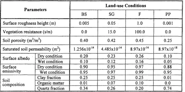
The soil domains in the four land-use conditions were assumed to be homogeneous and isotropic for the simplicity. The two vegetated elements (SG and F) and bare soil element correspond to real field scenarios while the porous pavement element may be slightly different from the real problem. Nonetheless, the simulation results are expected to be valuable either directly or indirectly in understanding redistribution and vertical migration behaviors of DNAPL contaminants in different land-use conditions. Some of the parameters, which characterized the four land-use conditions, are given in table 1.
Table 1 Parameters that characterized the land-use conditions
Land-use Conditions Parameters
BS SO F pp
Surface roughness height (m) 0.005 0.05 1.0 0.001
Vegetation resistance (s/m) 0.0 15.0 100.0 0.0
Soil porosity (m 3 /m 3 ) 0.40 0.42 0.45 0.25
Saturated soil permeability (m 2 ) 1.256xlO· 14 4.485xlO· 14 8.97xlO' 14 8.97xl0·
18Surface albedo Dry condition 0.20 0.23 0.26 0.10
Wet condition 0.10 0.12 0.16 0.05
Surface Dry condition 0.90 0.95 0.97 0.88
emissivity Wet condition 0.95 0.97 0.99 0.95
Soil Clay fraction 0.25 0.25 0.25 0.01
composition Organic matter 0.01 0.07 0.10 0.0
Quartz fraction 0.34 0.26 0.20 0.74
The unsaturated soil primarily consisted of five components: clay minerals, organic matter, quartz, liquid water and gases. The thermal, hydraulic and radiation properties depended on the proportions of these constituents. Porous pavement was assigned the smallest porosity value. The fraction of organic matter and porosity increased for vegetated land conditions as depicted in the table. The thermal heat conductivity in soil (A) was calculated using the following relation.
,\ ~ a(:')' + p(:} r (11)
where, ex, ~ and y are constants that were computed based on soil composition. TeE was adopted as a representative DNAPL in the simulation.
The flow velocities in both phases were assumed to be smaller in the unsaturated soil domain. The dimensionless Hemy's constant, latent heat of vaporization and diffusion coefficients in aqueous and gas phases were 0.236, 2.397 x lOs (Jlkg), 1.515 x 10. 9 (m 2 /sec.) and 6.94 x 10. 6 (m 2 /sec.) respectively (Sleep et aI., 1989). Most of the parameters used in the simulation were taken from literatures.
4. SIMULATION CONDITIONS AND COMPUTATION PROCESS 4.lInitial and Boundary Conditions
- 7 -
The atmospheric domain consisted of eleven uneven horizontally homogenous meshes.
The mesh size near the ground surface was the smallest and it increased towards the upper atmospheric boundary. The upper boundary was fixed at 3069-m from the ground surface, at which u = ug = 10 mis, v = V g = 0, 't x = 't y = 0, H = E = ° and 8elOz = O. Equations (4) and (5) governed for the surface boundary conditions. In addition to this, the summation of all the energy fluxes was equated to zero at the surface. Atmosphere was considered to be an infinite sink for DNAPL gas phase contaminant and its background concentration was assumed to be zero. The following relation was used for the transport of gas phase DNAPL at the ground surface.
E
jlrCT(g)= ,u{C
g(l) -C
g(a) }(12)
where, Etlux(g) = DNAPL gas flux at the ground surface (kg/m 2 -sec.), Cg(l) and Cg(a) are gas phase concentrations in the top soil layer and lower atmosphere respectively (kg/m 3 ) and /..l. is a coefficient for which a value of3.03 x 10- 8 (rn/sec.) was assumed in this simulation.
The soil domain was divided into twenty-five uneven horizontal meshes and the mesh thickness increased towards the depth. The meshes were taken to be homogenous and incompressible. The top of the water table was fixed at 1.62-m from the ground surface.
Initially, a uniform concentration of 1.10 and 0.40 kg/m 3 DNAPL in aqueous and gas phases respectively contaminated the top O.ll-m soil. Two cases of initial moisture content were taken into account. The first case consisted of completely unsaturated condition above the water table. The moisture content varied linearly from the top to its saturation value at the lower boundary. The second case considered a rainfall condition, which was represented by saturated liquid water content for the top 5-cm soil. Below this depth, the moisture distribution profile was the same as in the no rainfall condition. The total heat and liquid water fluxes at the lower boundary were equated to zero. Similarly, the convective fluxes of aqueous and gas phase DNAPL were equated to zero at this level.
4.2 Computation Process
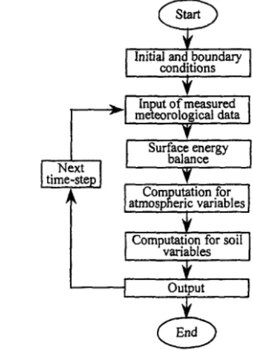
Fig. 2 Computation flow diagram in simulation
The computation procedure for the simulation is briefly outlined by the flow diagram in
figure 2. After imposing initial and boundary conditions, measured solar radiation, and air
temperature and pressure at screen height were given as input data. One-hour average of
these three parameters were obtained from a meteorological station in Hanno City, Saitama Prefecture. For every time step, the calculation started from surface energy balance, in which surface energy fluxes and surface temperatures were calculated. The computations for atmospheric and soil variables followed the sUlface energy balance. The computation process for a time step was repeated until a desired accuracy was obtained. The process ended when the designated simulation period was over.
5. RESULTS AND DISCUSSIONS
This simulation was carried out for five days duration. The input data (from July 5 to 9, 1998) of solar radiation, and air temperature and pressure at a screen height were the same for all the cases considered in this paper. Partitioning of the solar radiation into four different surface energy fluxes (sensible heat, latent heat of vaporization, net radiation and ground heat) was an important point in the simulation. Differences in the representative surface radiation propeliies for the land-use conditions mentioned in this paper resulted to variations in surface energy fluxes. Similarly, different soil compositions, porosity and soil hydraulic and thermal properties led to differences in heat, moisture and contaminant migration behaviors in unsaturated conditions in the shallow subsoil. The simulation results are discussed in the following sections for the four land-use cases in two different moisture saturation conditions in terms of surface energy fluxes, soil heat and moisture budgets and DNAPL transport behavior in the subsurface. Only the significant results are shown in figures.
5.1 Suiface Energy Fluxes
o
96 120
48 72
Simulation time (hrs.) 24
·100
.200
c...;.".~..ILU.";"""'''''''''';:.-h!.L...J::.J..w.~...~~...:I120 a
96
48 72
Simulation time (Ius.) 24
400
He ! 300
.. ~ 200
~ 5
i 100
Vl
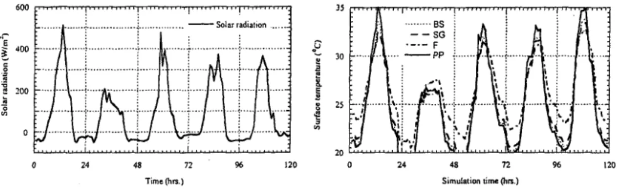
Fig. 3 Surface energy fluxes for porous pavement (no rain) Fig. 4 Surface energy fluxes in forest (no rain) Figure 3 and 4 respectively show surface energy fluxes for porous pavement and forest elements in no rainfall condition. The incoming solar radiation shown in figure 5 and the simulated energy fluxes indicated that the second simulation day was cloudy and the remaining four days were sunny. Porous pavement and forest respectively exhibited the highest and the lowest daytime maximum net radiation flux values. Bare soil and short grass respectively showed the second and the third highest values. The average daytime maximum values for bare soil, short grass and forest were respectively about 94%,86% and 76% of the corresponding value for porous pavement case. But, the nighttime maximum values were just in the reverse order due to increasing emissivity coefficient However, the order of fluctuation between day and nighttime net radiation values was the same as that of daytime maximum values. The daytime maximum values slightly decreased in rainfall condition
- 9 -
compared to the conesponding no rainfall cases. On the other hand, nighttime maximum values increased due to increasing emissivity in wet condition. However, the effect of rainfall seemed to decrease in the later part ofthe simulation.
120
9672 48
24
20
u..u..~u.UJLU.L~-U.l!:I:w..s...u.w..u.ill ...~...u!Cw.L...uJo
120 96
72
." - Solarradialion . ,_ .. B5
t
~30 •. ", ...
- p p'-'- --SG F
I .e 8 25 'l!
~'"
24 48
Time (hrs.) Simulation time (hrs.)
Fig. 5 Incoming solar radiation in the simulations Fig. 6 Surface temperature profiles for the land elements
Porous pavement and bare soil showed bigger latent heat fluxes in daytime compared to vegetated surface probably due to direct influence of the incoming solar radiation resulting to increased evaporation. The average daytime maximum latent heat fluxes for bare soil, short grass and forest respectively were about 97%, 87% and 41 % of the porous pavement case. At night, the non-vegetated surfaces exhibited very small latent heat fluxes compared to vegetated surfaces. This could be attributed to vegetation transpiration. Between the two vegetated surfaces, forest showed higher values compared to short grass case at night. In terms of fluctuations in latent heat during a day, porous pavement, bare soil, short grass and forest elements were in the decreasing order. .
With respect to daytime maximum sensible heat flux, the four land elements were in the reverse order as in the case of net radiation flux. The sensible heat flux increased for vegetated surface due to increase in surface albedo values. These fluxes slightly decreased in rainfall condition since albedo values in wet condition were smaller than in dry condition.
However, this effect disappeared in the later part of the simulations.
Between the two non-vegetated swfaces, bare soil showed bigger values of daytime maximum ground heat flux. It slightly decreased in vegetated smfaces. The results indicated that the ground heat flux decreased for increasing vegetation density. The effect of rainfall was to increase this heat flux. However, this effect was more distinct in vegetated surfaces than in non-vegetated one.
5.2 Soil Heat and Moisture Budgets
Figures 7 and 8 show soil temperatme profiles at four different depths from the ground surface in porous pavement and forest elements respectively for the total simulation period in no rainfall condition. The effect of cloudy weather on the second simulation day resulted to smaller temperature values compared to that in other days. It is first attempted here to discuss the simulation results for soil temperature distribution in terms of surface temperature variations. The surface temperature variations for the four land-use conditions are shown in figure 6.
During the simulation period, the maximum surface temperature fluctuations for all the land-use conditions remained between 17°C and 35°C. Porous pavement, bare soil, short grass and forest elements were in decreasing order with respect to daytime maximum surface temperature. The last three elements in this case exhibited about 96%, 95% and 93%
maximum surface temperature of the values for porous pavement case respectively.
Nighttime minimum surface temperatures were in the reverse order. For all the four
conditions, the minimum surface temperature in a day increased as simulation progressed.
The daytime maximum values seemed to decrease in rainfall. condition, but it was not significant.
96 120 72
48
Simulation time (hrs.) - - O.2·em
24
·..,····..·...1··...·....:..·...····.. +....·..·..····
32
"-' G
!!~
28
i! 8-
.!!
E
·0
24
<Il
20
96 120 0
32
1\ - - O.2·em
!....
It ···-··S.O-em
"'- G 28 a
~"
~ Co.!!E
0 24
<Il
20
0 48 72
Simulation time(hrs.)
Fig. 7 Soil temperature profiles in porous pavement (no rain) Fig. 8 Soil temperature profiles in forest (no rain)
As depicted in figures 7 and 8, the top 5-cm soil was the most affected by diurnal fluctuations in solar radiation. However, the effect reached up to 40 to 50 cm depth during the simulation. There were successive time lags for the same events (for example: maximum or minimum temperatures) at different soil depths due to the time lapsed for heat transport from one layer to the underlying layers. Even though the surface temperatures were relatively smaller for vegetated land-use conditions in the afternoon, a close observation on these figures indicated that vegetated subsurface exhibited relatively bigger temperature. For example: the soil temperatures at 15-cm soil depth at the end of the five-day simulation for forest and porous pavement were about 25°C and 24°C respectively. Similar behavior could be observed at other depths and times. Relatively bigger initial moisture content and higher percentage of organic matter content for the vegetated subsurface might have resulted to bigger thelmal heat capacity, ultimately giving rise to bigger subsurface temperature. This behavior of vegetated subsurface could have significant impact on aqueous phase DNAPL migration, which will be discussed little later. In case of rainfall condition, not any significant changes in subsurface temperature were observed due to its short duration.
The liquid water content profiles at four different soil depths for no rainfall condition in bare soil and forest cases are depicted in figures 9 and 10 respectively. The soil moisture content in the topsoil sharply increased during the first simulation day for all the four cases probably due to small initial moisture contents. This trend remained unchanged till later in bare soil case although the rate of increase was less sharp compared to the earlier days. In case of short grass, the diurnal fluctuations dominated the continuous increasing trend from the second simulation day. For forest element, both of these trends disappeared and the moisture content gradually decreased till the end of the simulation from the second day.
Porous pavement case showed similar trend with short grass, but the changes in moisture content were not smooth. They exhibited rather stepping nature. Smaller porosity value and other soil properties could have resulted to such a behavior. Similar to soil temperature, the effects of diurnal changes in solar radiation were reflected most significantly in soil moisture content in the top 5-cm depth. Bare soil and forest elements respectively exhibited the maximum and the minimum moisture fluctuations in the topsoil during a day. Short grass and porous pavement elements showed the second and the third highest fluctuations respectively.
The results indicated that vegetation cover significantly affected the moisture distribution in
-11-
the top unsaturated zone. Decrease in moisture fluctuations were observed from bare soil to short grass and from short grass to forest cases. As the effect of vegetation increased (forest), the soil moisture continuously decreased in the later part of simulation most probably due to increased vegetation transpiration.
Simulation time (hrs.l
120 96
- -0.2-em ---··S.O-em
"!"""""",,,,! ..
~... - - - ·;0 -1S.0-cm
(l·co: ..24 48 72
Simulation time (hrs.l
'0(I)
0.28
-:s 0.36 _ ...
i :8~ 0.32
I :j 0.32 ···..···.. ···f····..····.. ~>~~~,"r~~~...,~~···~i:.~·
':: 5 'I : ",r:::~' ! ,... - - 0.2 cm ..
1: , . : ----5.0 cm
8 "i : -15.0em
II 0.28 .1..; , -400Clll .
';l
r'; : ;
i 0.26 ·/~! .... j...••.•• ....j. ...1•.·.••••••••••• 1.
: : : :
Fig. 9 Soil moisture profiles in bare soil (no rain) Fig, J 0 Soil moisture profiles in forest (no rain) The moisture content profiles in these two cases (bare soil and forest) in rainfall condition are shown in figures 11 and 12 respectively. The order of maximum moisture fluctuation in the topsoil during a day was the same as in no rainfall condition. But the fluctuations in this case were smaller than in no rainfall condition for all the elements. Since the top 5-cm soil was initially saturated with liquid water in representing rainfall condition, the moisture content in this area sharply decreased in the first I2-hrs simulation due to percolation.
However, this trend was not observed in porous pavement case and that was similar to its no rainfall condition, As in no rainfall condition, moisture content below I5-cm depth gradually decreased in vegetated elements. But the decrease seemed to be faster compared to no rainfall condition in the later part of the simulation probably due to increased vegetation transpiration.
120 96
72 24 48
0.32 u...
...J~~...L~~'-'-'-'-'...u.L...u..LU..Jo
1: 0.38
I I 0.36
"
'C
~ _ 0.34
'0 >-
96 120 72
24 48
0.29 ...
~...,,~...
...J..,...~...""--'-"~...o
-i 0.3S 1'" ; , , : ..
! o·"·lt.=;~vr\t
! :::: ::·.···::···:.·.1~~~~[·.··:::.\~~.·.r .. ::··.~~ .. ·J::.::::.~ ...:::
.~ J i - - 0.2-em i
II .,'\ .1 i ._- ;.0-,,,, :
§ 0.31 ....
\:~'T.. r·....·...·..· -IS.O-em ....·..·.. ·1..·..·...·
~ \j i - 40.0·on i
03 ·..· ··· .. t· ·.. ·t·· ·r···..··..··..·.. r··· ··..
Simulation time (hrs.) Simulation time (hrs.)
Fig, 11 Soil moisture profiles in bare soil (rain) Fig. 12 Soil moisture profiles in forest (rain)
5.3 Aqueous Phase DNAPL Migration Behavior
The top II-em soil was initially contaminated with aqueous and gas phase DNAPL and
the diurnal soil moisture and temperature fluctuations were significantly bigger in the top 15-
cm depth. Therefore, it would be relevant to discuss the simulation results in two stages: the concentration distribution behaviors in the contaminated soil layer and below it.
0.3
-...~...
...,.'-'-'-'-'~...
u..u..~...~...~""'-"o 0.2 0.4 0.6 0.8 I . 1.2
Aqueous phase DNAPL concentration (kgilrl') Aqueous phase DNAPL concentration (kgln{) 1.2 0.8
0.6 0.2 0.4
i - - I-hrs - 18-l1rs ~ 60-hrs
...+ --2·hrs -24·hrs
--~-lll' ....i
- 0 -3·hrs - 30-hrs - 84-hrs
i - - 5·hrs - - 36·hrs . - • - . 96-hrs
...L. -?·hrs -42-hrs --108·hrs
: -9-hrs -48·hrs J20-hrs
! - 12·hrs - - 54·hrs 0.06
! 0.12
a ..
'0
'0
0.18
en
0.24
0.3 0
;
~I-IllS -18·hrs -60-hrs
...+
~2-hrs-24-hrs
--~.'·hl'i
- a -3-hrs - 30-hrs - 84-hrs
i - - 5-hrs - - 36·hrs -. - - . 96·hrs
;
~7·hrs -42·hrs -108·hrs
···1· ~9·hrs -48·hrs ···120-hrs
i
~12·hrs - 54-IllS 0.24
0.06
'0 0.18
'"
! 0.12
..r::
t
Fig. 13 Aqueous concentration in forest (no rain) Fig. 14 Aqueous concentration in porous pavement (no rain)
Figures 13 and 14 show aqueous phase concentration profiles in the contaminated soil layer for forest and porous pavement elements respectively in no rainfall condition. The concentration decreases were relatively bigger in the first 12-hrs simulation in all the cases due to small~r initial moisture content resulting to rapid increase in this parameter during this period. Bare soil, short grass and porous pavement showed decreasing tendency in concentration towards the surface from the middle of the contaminated layer. But, it sharply increased from 12-hrs onwards, which might indicate the increased evaporation from the surface. During the simulation, the first afternoon exhibited the maximum solar radiation and the non-vegetated elements showed relatively sharp increase in aqueous phase DNAPL concentration, which might strengthen the idea of increased evaporation. In forest element, this concentration increase in the topsoil layer started right from the beginning probably due to increased transpiration compared to short grass case. The concentration profiles near the bottom of the contaminated layer smoothly decreased to their minimum values. The aqueous phase concentration decreases in this soil layer during the five days simulation were more than 95% in all the cases considered.
The overall concentration decrease in the contaminated soil layer in rainfall condition was relatively slower compared to the corresponding cases in no rainfall condition. Higher soil moisture content in the topsoil due to rainfall might have reduced DNAPL volatilization resulting to the slower decrease rate in aqueous phase concentration. However, the concentration decreases just below the contaminated layer were sharp in this case unlike the relatively smoother trend in no rainfall condition.
The aqueous phase concentration profiles in forest and porous pavement elements below the contaminated soil layer in no rainfall condition are depicted in figures 15 and 16 respectively. As simulation progressed, the concentration fronts moved to deeper soils in all the cases. Comparing all the four cases, the vertical migration depths of aqueous phase DNAPL were the highest and the lowest for forest and porous pavement respectively. The short grass and bare soil showed the second and the third highest values respectively. For instance, let us have a look of the maximum concentration depths below the contaminated layer at two different times of the simulation. At 96-hours, porous pavement, bare soil, short grass and forest elements showed maximum aqueous phase concentrations at 0.21, 0.25,0.26 and 0.37-m depths from the surface respectively. Similarly, the migration depths for the elements in the same order at 120- hours were respectively 0.27,0.35,0.36 and 0.47-m. The
-13-
migration depths below the contaminated layer were less distinct among the elements in the begilU1ing of the simulation. Bare soil and short grass showed similar vertical migration depths compared to other elements in spite of increase in soil porosity and initial moisture content for the latter. This behavior could be attributed mostly to the vegetation resistance to gas flow,which was smaller in short grass case compared to forest element.
• - - J-hrs - IS·lm
~60-hrs... --2·hrs -24-hrs -";·lir·, - - 3-hrs - 30-hrs - S4-hrs - - S-hrs - 36-hrs _•• - . 96-hrs 0.9 ..::::::;,.::::::::::: =~:~~ =:;:~::::::::: :~~:::
--12·hrs -54-hrs
1.1 ... .=.L...
u.W..<.~.w...~...u.W..<...u..u...a
o 0.01 0.02 0.03 0.04
Aqueous phase DNAPL concentration (kgln{) '0 0.7
en
g 0.5
!
0.01 0.02 0.03 0.04
Aqueous phase DNAPL concentration (kgln{) - J8-hrs
~60-hrs-24-hrs
-'.~·I,,·- 30·hrs - 84·hrs - 36-hrs ••. - . 96-hrs .: ... ~ ...l ~ 7-hrs - 42.hrs .,._- 108-hrs
/..t : ~ 9·hrs - 4S·hrs J20-JU'S
.;f '1' ~ 12·lm - S4·hrs
'.,"
.
O'J~ii""'~
0.3
....
~ _ ~.
t
~
1.1 o
0.9
~ 0.5
i
'00.7
Vl
Fig. 15 Aqueous concentration in forest (no rain) Fig. 16 Aqueous concentration in porous pavement (norain)
The concentration profiles below the contaminated layer for forest and porous pavement
in rainfall condition are shown in figures 17 and 18 respectively. The land elements were in
the same order in terms of vertical DNAPL migration depths as in no rainfall case. The
depths of maximum concentration at 96-hours of simulation for porous pavement, bare soil,
short grass and forest were 0.12, 0.14, 0.21 and 0.32-m respectively. These depths at the end
of the simulation were respectively 0.24, 0.28, 0.31 and 0.42 meters. This scenario indicated
that the depths of maximum concentrations at any time along the vertical soil profile in
rainfall condition were relatively smaller than in no rainfall condition. For instance, the
depths of maximum concentration at the end of the simulation in forest element in rainfall
and no rainfall conditions were respectively 0.42 and 0.47 meters. At the same time, the
maximum concentrations at any time below the contaminated layer increased in rainfall
condition than that of the corresponding cases in no rainfall condition. As for example,
porous pavement and forest in no rainfall condition showed only 50% and 65% maximum
concentrations of the corresponding rainfall cases at the end of the simulation. These results
again might strengthen the idea of reduced volatilization in topsoil in rainfall condition as
discussed in the earlier paragraph. On the other hand, the maximum depths of aqueous phase
DNAPL migration increased in rainfall condition compared to no rainfall condition. For
instance, the concentrations at 1. I O-m depth for porous pavement, bare soil, short grass and
forest elements in no rainfall condition were about 33%, 60%, 69% and 72% of their
respective values in rainfall condition. The initially saturated topsoil in rainfall condition
might have played dual roles in this context. It might have reduced the interaction between
the surface and the subsurface in terms of soil temperature and moisture fluctuations, which
might have resulted to reduced DNAPL volatilization. At the same time, it provided enough
moisture for percolation resulting to deeper DNAPL migration in aqueous phase. The
downward migration process might have been enhanced further in vegetated elements due to
their bigger porosities, relatively bigger initial moisture contents and shielding effect for the
incoming solar radiation.
0.01 0.02 0.03 0.04 Aqlleous phase DNAPL concentration (kgln?)
0.04 0.03
,..·...·!··..·.... ·I·:::::::::r.:::·::::
0.02 0.01
Aqueous phase DNAPL concentration (kgln?) . 'I - I·hrs - 18·hrs
~60-lus
1:;!.f; -
2..hrs - - 24-hrs - - -:
-Ill"",...: ...,- 3-hrs - 30-hrs - - 84-hrs
! --- 5-hrs - - 36-hrs - - - - . 96-rhs
r--..·.... 1 -7-hrs -42-hrs --108-hrs : : -9-hrs -48-hrs ....·.... 120-hrs ..., ; - 12·hrs - 54-hrs
: :
1.Iu..u.u..J~...L~...L...
....w..-..=...
~...w.....w...
o
0.9
O'I~~
0.3r~
g 0.5
.,.n~7'-~··:.>'!
'00.7
til '
..
..
,:.
. - - 1·lus - 18·hrs - 60·hrs
./.:$ - - 2·hrs - 24·hrs - - ,
:-lLr·,, - a - -
3.hrs - 30-hrs - 84·hrs
.
~- - - 5-lus - - - 36-hrs - - - - . 96-lus
... 'J;?': -7·hrs - 42-hrs - " 108-hrs . ,:.:.': -9·hrs -48-hrs 120·hrs
"",.;,: ... ; 12 h 54 h
I)~:~: ~- - rs ---- • rs 0.1
0.3
g 0.5
.cC.
'0u
'0
0.7
til
0.9
1.1 0
Fig. 17 Aqueous concentration in forest (rain) Fig. 18 Aqueous concentration in porous pavement (rain)
5.4 Gas Phase DNAPL Migration Behavior
0.08
!
···[···:·;···r
0.02 OM 0.06
Gas phase DNAPL concentration (kgln?) : -I-hrs --18-hr. --60-hrs
..+ -2-hrs ~-24-hrs--'2-llI"s
!
- a - -3.hrs - 30-hr. - - 84-hrs
: - - 5·hrs - - 36-hr. - - - •. 96-hrs
j
!.. -7-hrs --42-hrs ---108-hrs
i
j-9·hrs -48-hrs J20-hrs
j i - 12-hrs - 54-hrs
0.1
0.2
:§:
.;: 0.3
~Co
~
'" 0.4
0.5
0.6
0.1 0
Q~ Q~ Q~ QOO
Gas phase DNAPL concentration (kgln?)
. i - I-hrs - - - 36-hrs
.: ... ..i... i... - 2-hrs -42-hrs
• : - 0 -
3-hrs - 48.hrs
.. ·-j--... !·..·.... I..·.. -- ~:~~ ~~:~
: : : -12-lus -84-hrs
...f... ~ ... ..+... -18-hrs ---96-hrs
: : : - 24-hrs - - 108-hrs
: i i - 30-hrs ... 120-hrs
: : :
o
0.1
0.2
!
.c C.0.3
'0u
:a '" 0.4
0.5
0.6 0
Fig. 19 Gas concentration in forest (no rain) Fig. 20 Gas concentration in porous pavement (no rain)
Figures 19 and 20 show DNAPL gas concentration profiles for forest and porous pavement elements respectively in no rainfall condition. The gas concentration gradually decreased towards both the vertical directions from the bottom of the contaminated layer in all the elements. More than 90% gas phase contaminant decreased within the first 12-hours simulation probably due to the contaminant being present at the top of the soil domain.
Another important reason for such drastic changes in gas phase concentrations could be the initial low moisture content and its quick redistribution in the first twelve hours period, as was discussed in the earlier section. The maximum concentrations at 12-hrs were observed at 0.09-m depth in all elements unlike the case in aqueous phase concentration. Not any such distinct trend in terms of gas phase concentration decrease was observed in the contaminated layer among the land-use conditions like in aqueous phase concentration distributions.
However, the results indicated that the decreases were relatively bigger in vegetated elements, There could be two possible ways of gas phase contaminant decrease in the contaminated layer. The first one was to escape to the atmosphere and the second was to migrate to deeper soils. In vegetated elements, the vegetation resistance could impose some restriction to gas phase contaminant movement to the atmosphere compared to non-vegetated cases in addition to their relatively bigger porosity. This might indicate that relatively higher fraction of gas
-15-
phase contaminant migrated to deeper soils in vegetated soils. On the other hand, DNAPL volatilization might have contributed to more gas phase contaminant in the contaminated layer of the non-vegetated elements since they exhibited bigger temperatures. This could have resulted to the relatively smaller concentration decreases in these elements.
0.024
..···....·j··.. ··.. ·i.. ···:::::r::::::::·r::::::
0.006 0.012 O.Q1S
Gas phase DNAPL concentration (kgl.rl)
.... ---!·hrs -18·hrs
~60-hrs... - - - 2·hrs - - 24-hrs -
'.~·h".. - - a -
3·hrs - - 30-hrs - 84·hrs
....1 · --- S·hrs - - 36·hrs ..••. 96-hrs
...1...
~7-hrs - 42-hrs - - J08·Jus
~
9·hrs - - 48-hrs ... 120-hrs ... - 12-hrs - - 54·hrs
O.l
0.3
~ 0.5
-"
is.
u"0
'0
0.7
til
0.9
1.1 0 0.024
....
~..
, ~. i ···f····..····I···t···..I··..···
0.006 0.012 0.018
Gas phase DNAPL concentration (kglm)
~
1·lus - 18·hrs
~60·hrs
;
-2~hrs- 2 4 hrs -7>11·,.
i
~-3-hrs - 30·hrs - 84-hrs
·1 ·..·..· ...- S·hrs
~36·hrs • - ••. 96-hrs
... ;
~7-hrs - 42-hrs - !08-hrs
i - 9 - h r s -48-hrs 120·hrs
....j - 12-hrs - S4·hrs
0.1
0.3
:§: 0.5
a
u"0
:a 0.7
'"
0.9
J.l 0
Fig. 21 Gas concentration in forest (no rain) Fig. 22 Gas concentration in porous pavement (no rain)
The gas phase concentration profiles below the contaminated soil layer in no rainfall condition for forest and porous pavement are depicted in figures 21 and 22 respectively.
From these figures, it is more clear that the concentration decreases were faster in vegetated element. For instance, the maximum gas phase concentration for forest at 72-hours was about 77% of the corresponding maximum value for porous pavement. Similarly at the end of the simulation, the maximum concentration for the former was about 70% of the latter. In terms of vertical migration depth in gas phase, forest and porous pavement showed the maximum and the minimum values respectively similar to the trend in aqueous phase. Short grass and bare soil were in the second the third places even though there was no such clear distinction between these two elements. As for example, porous pavement, bare soil, short grass and forest elements showed the maximum gas phase concentrations at 0.34, 0.40, 0.41 and 0.49- m soil depths respectively at the end of the simulation. Thus, the gas phase contaminant vertical spreading was significantly bigger than in dissolved phase.
In rainfall condition, the four land-use conditions exhibited similar tendencies as were in no rainfall condition with respect to gas phase contaminant transport. The concentration profiles below the contaminated soil layer in rainfall condition for forest and porous pavement are shown in figures 23 and 24 respectively. Similar with aqueous phase, .the depths of maximum DNAPL gas concentrations decreased in rainfall condition compared to the corresponding no rainfall cases. For instance, the depths of maximum concentration for forest at 72-hours in no rainfall and rainfall conditions were 0.32 and 0.29 meters respectively.
Similarly, these values at the end of the simulation were 0.49 and 0.47 meters. On the other
hand, the maximum gas concentrations in rainfall condition increased. These values at 120-
hours in no rainfall condition for porous pavement, bare soil, short grass and forest were
about 47%, 58%, 64% and 66% of the corresponding values in rainfall condition. These
scenarios of gas phase concentrations might imply that the initially saturated topsoil layer
played a vital role in two ways. In one hand, it might have reduced the interaction between
atmosphere and soil resulting to smaller depths of maximum concentrations. On the other
hand, the saturated soil cap reduced the escape of gas phase contaminant into the atmosphere
resulting to the increase in the maximum concentration values in the soil domain.
0.024
·t~_···
...j" + -j-- i ..
0.006 0.012 0.018
Gas phase DNAPL concentration (kglrrt) 0.3
1.1 ...u-W~.w...~u....~
...
~"'-'-'-...,
o 0.9
i - I-Ill'S - 18-11rs - 60-hrs
~
0.7 ... ... !. -2.hrs -24·hrs
--:-hl':....l
- a -3-hrs - 30-hrs - 84·hrs
; i - - 5-hrs - 36·hrs • - - - . 96-hrs
...L...). -7-hrs - 42·hrs _••_- IOS-hrs
i i - 9-hrs - 48·hrs ... 120-hrs
... ( ...1' - 12-hrs - 54·hrs
~ 0.5 .c ~
0.024 0.018
0.012 0.006
Gas phase DNAPL concentration (kglnf) - I · h r s -18-hrs -60-hrs ... -2-hrs -24-rhs
- " . ' · I i "- a -
3-hrs - 30-hrs - 84-hrs
... - - 5·lus - - 36-hrs •• - - . 96-hrs
1 - 7·hrs - 42-hrs '--'108-hrs - 9-hrs - 48-hrs ....···120-hrs
.• j •••...