The Effects of Capital Taxation Using Dynamic Macro-Econometric Model of the Japanese Economy ―Simulation Analysis Including Households without Financial Assets―＊

The Effects of Capital Taxation Using Dynamic Macro-Econometric Model of the Japanese Economy

―Simulation Analysis Including Households without Financial Assets―

^＊

Daisuke Ishikawa

Former Senior Economist, Policy Research Institute, Ministry of Finance

Dun-Yen Wang

Researcher at the Research Center for Advanced Policy Studies, Institute of Economic Research, Kyoto University

Masahiko Nakazawa

Visiting Scholar, Policy Research Institute, Ministry of Finance

Abstract

In order to maximize social welfare, it is important to ensure stable economic growth by revitalizing private-sector. From this viewpoint, it is necessary to design capital taxation such that it avoids undue distortions in the corporate sector as much as possible. On the oth- er hand, as the government’s fiscal situation is deteriorating, reform on tax system must also be consistent with fiscal sustainability. With these perspectives in mind, we developed a dy- namic macro-econometric model (dynamic CGE model) that contributes to the analysis of capital taxation, in reference to Radulescu (2007) and Radulescu and Stimmelmayr (2010), while including households without financial assets. In this paper, we report the results of various numerical simulation analyses, maintaining neutrality of tax revenues.

　 Keywords: dynamic macro-econometric model, capital taxation, liquidity-constrained consumers, tax revenue neutrality

　 JEL Classification: C54, H21, H25

* The opinions expressed in this paper do not necessarily reflect the views of the organizations which they belong to. We

would like to express our appreciation to: the following individuals and people who participated in the following events for the

valuable suggestions and comments that they contributed to the preparation of this paper: individuals: Hirokuni Iiboshi, (Pro-

fessor, Tokyo Metropolitan University), Hisakazu Kato (Professor, Meiji University), Masumi Kawade (Professor, Nihon Uni-

versity), Sumio Saruyama (Lead economist, Japan Center for Economic Research), Takero Doi (Professor, Keio Univeristy),

Toshiki Tomita (Professor, Chuo University), Masaki Nakahigashi (Associate professor, Niigata University), Ryo Hasumi (Re-

searcher, Japan Center for Economic Research), Makoto Hasegawa (Associate professor, National Graduate Institute for Policy

Studies), Toshiya Hatano (Professor, Meiji University), Naoyuki Yoshino (Professor Emeritus, Keio University), and partici-

pants in the autumn 2015 meeting of the Japanese Economic Association (Sophia University), the 2014 meeting of the Japan

Institute of Public Finance (Chukyo University), the eighth Macro Model Seminar (Japan Center for Economic Research, Sep-

tember 2014), the CAPS seminar (Institute of Economic Research, Kyoto University). Of course, the authors are solely respon-

sible for any errors.

I. Introduction

In order to maximize social welfare, it is important to ensure stable economic growth by revitalizing private-sector. From this viewpoint, it is necessary to design capital taxation such that it avoids undue distortions in the corporate sector as much as possible. On the oth- er hand, as the government’s fiscal situation is deteriorating, reform on tax system must also be consistent with fiscal sustainability. With these perspectives in mind, we developed a dy- namic macro-econometric model (dynamic CGE model) that contributes to the analysis of capital taxation, maintaining neutrality of tax revenues.

Among previous studies concerning capital taxation using a dynamic macro-economet- ric model (dynamic CGE model) are Radulescu (2007) and Radulescu and Stimmelmayr (2010). Radulescu (2007) and Radulescu and Stimmelmayr (2010) conducted numerical simulations using a dynamic macro-econometric model with respect to the capital tax re- form programs in Germany (including dual income taxation). This paper seeks to extend the models in Radulescu (2007) and Radulescu and Stimmelmayr. Let us explain the salient characteristics of our model. First, we designed the corporate sector in more detail compared with other studies. Specifically, (1) various means of financing (retained earnings, new debts and new equity issuance) are embedded in the model, (2) an agency (risk) premium is en- dogenously determined in a debt interest rate, and (3) the model formulates allowance for corporate equity (ACE) and allowance for net investment (accelerated write-off) in the tax bases.

Second, we introduced heterogeneity in the corporate sector. Specifically, the model in- cludes (1) PIH consumers who have financial assets and can afford intertemporal consump- tion smoothing in accordance with the Permanent Income Hypothesis, and (2) LIQ consum- ers who face a liquidity constraint and cannot build up savings.

Third, we constructed a two-country open economy model, incorporating the current ac- count balance and net foreign assets. Specifically, (1) the trade balance is endogenously de- termined in such a way that domestic investments and savings are balanced, and (2) a full home bias is assumed with respect to stocks and corporate bonds while domestic and foreign government bonds are internationally traded.

This paper contributes to the literature by analyzing an economy in which the LIQ con- sumers, who do not have financial assets and cannot afford intertemporal consumption smoothing, are explicitly embedded: the LIQ consumers are not subject to interest income tax, income gain tax and capital gains tax. Therefore, the macro-economic effects of impos- ing these taxes may be affected by the heterogeneity of the household sector.

¹

Previous stud- ies, such as Radulescu (2007) and Radulescu and Stimmelmayr (2010), conducted their analyses using models including only PIH consumers with financial assets, whose behavior follows the Permanent Income Hypothesis.

1

In the long term, these taxes will affect the accumulation of capital stock. That, in turn, will have secondary spillover effects

on LIQ consumers through changes in their wage rate.

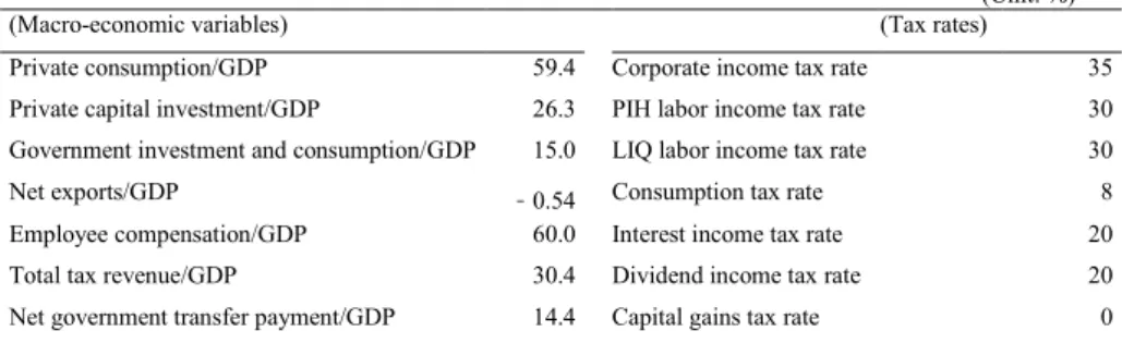
Examples of policy analysis in this paper include: “analysis of how taxation affects mac- ro-economic variables (GDP, effective marginal tax rate, capital cost, capital stock, debt ra- tio, labor supply, effective wage rate, consumption, social welfare, etc.,” “analysis of dual income taxation,

²

” “analysis of allowance for corporate equity (ACE) in the corporate tax base and net investment allowance (accelerated write-off),” and “analysis concernin the

“New View” related to finance.

³

”

This model can implement various simulations which contribute to solve policy chal- lenges we face, while based on specific calibrations.

The rest of this paper is as follows. Section 2 explains the theoretical structure of the dy- namic macro-econometric model that contributes to the analysis of capital taxation. Section 3 explains data and calibration of parameters. Section 4 shows the simulation results. Sec- tion 5 summarizes the findings of this paper.

Ⅱ. Theoretical models

II-1. Assumptions of the model

⁴

II-1-1. Normalization of variables and long-term path of balanced growth (steady- state equilibrium)

We assume that the Japanese and overseas economies have a constant technological progress rate expressed as 1+tech = X

_t+1

/X

_t

(X

_t

: level of labor-augmenting technological progress) and a population rate expressed as 1+n. We also assume that as in the case of Ku- mof et. al. (2010), the variables in the model are normalized by the technological progress level X

t

and the population growth rate (1+n)

^t

.

⁵

The normalized variables thus converge to time-invariant constant values in the long-run equilibrium (steady state). Hereafter, the gross economic growth rate is expressed by the equation G ≡ 1+g = (1+tech)(1+n) (g=net eco- nomic growth rate) while the time index is dropped from the variables in the steady state.

II-1-2. Assets and their rates of return

Outstanding of stocks and bonds and their rates of return are as follows: stocks V are is- sued by domestic corporations (after-tax rate of return r

^V

); debts B are issued by domestic corporations (pre-tax rate of return excluding the premium i

^BH

); sovereign bonds D

^GH

are is- sued by the home government (pre-tax rate of return i

^H

), stocks V

^F

are issued by foreign corporations (after-tax rate of return r

^VF

); sovereign bonds D

^GF

are issued by foreign govern- ments (pre-tax rate of return i

^F

).

2

Under dual income taxation, given that capital is more mobile than labor, labor income is progressively taxed while capital income is taxed at single rate lower than the lowest tax rate applied to labor income.

3

According to the New View, widely accepted in the field of corporate finance theory, net investment is financed by retained earnings and new borrowings in a developed economy, without the involvement of new equity issuance (η=0). (Auerbach (1979); Bradford (1981); Sinn (1987))

4

The theoretical model discussed herein much owes to Radulescu (2007).

5

Variables related to labor are normalized only by (1+n)

^t

. The rate of return and the wage rate are not normalized.

This model assumes complete home bias in stocks and bonds issued by corporations.

Therefore, stocks and bonds issued by domestic corporations are held only by domestic resi- dents while stocks and bonds issued by foreign corporations are held only by foreign resi- dents. In addition, it is assumed that portfolio selection across these asset classes is made under imperfect substitution, with the rates of return allowed to vary across them (Goulder and Eichengreen (1992)). However, we assume perfect substitution between sovereign bonds issued by the home and foreign governments (i

^H

= i

^F

).

Denoting the tax rate on interest income as τ

ⁱ

, the after-tax rates of corporate and gov- ernment bonds in the domestic fund investment sector (household sector) is calculated as follows, based on the residence principle of taxation: the after-tax rate of return on bonds is- sued by domestic corporations is expressed as r

^BH

≡ (1 − τ

ⁱ

) i

^BH

, while the after-tax rate of re- turn on sovereign bonds issued by the home government is expressed as r

^H

≡ (1 − τ

ⁱ

) i

^H

. The after-tax rate of return on sovereign bonds issued by foreign governments is represented by the equation r

^F

≡ (1 − τ

ⁱ

) i

^F

.

II-2. Corporate sector

II-2-1. Assumptions in the corporate sector

We assume a linear homogenous CES (Constant Elasticity of Substitution) production function incorporating capital and labor as follows (eq.(1)):

Y

t

＝F （K

t

, L

t

）＝A

t

d （L

t

） ＋（1－d）

^－1－ξξ

（K

t

）

^1－ξ

－ ξ 1－ξ

－ξ

(1)

where Y

t

= value added of the production; K

t

= capital stock at the beginning of the date t; L

_t

= the labor input; A

_t

= standardization coefficient; d: the parameter concerning factor input share; ξ: the elasticity of subustitution concerning factor inputs.

Capital stock is determined by the Q-theory discussed by Tobin (1969), and Hayashi (1982), etc. Smoothing of capital spending over time is characterized by the adjustment cost convex function J (I

_t

, K

_t

). The adjustment cost function J

_t

satisfies the conditions J

_I

> 0, J

_II

>

0, and J

K

< 0 and is homogenous of degree one, thus converges to 0 in the steady state.

⁶

I

t

represents the amount of investment.

We assume that retained earnings and issuance of new debts and shares are financing in- struments in the corporate sector. Regarding debt finance, we assume that a risk premium goes up as the corporate debt ratio rises. The agency cost function m(b) that determines the risk premium is formularized as a convex function, satisfying the conditions m′ > 0 and m″ >

0 as shown below (Strulik (2003)).

m

t

＝m （b

t

）＝ m （b

1 t

－m

2

）

²

b

t

, b

t

≡ B

t

K

t

(2)

6

Differential J

I

and J

K

also converges to 0 in the steady state.

where b

t

: debt ratio; m

1

and m

2

: the coefficient concerning the agency cost function (m

1

>

0, −1 < m

₂

< 1); B

_t

: the debt amount at the beginning of date t.

II-2-2. Calculation of corporations’ after-tax profits, corporate tax and dividend payouts

Typical corporations’ after-tax profit π

_t

and the corporate tax amount T

^P_t

are given as fol- lows:

π

t

= Y

t

− J

t

− w

t

L

t

− δK

t

− (i

^BHt

+m

t

)B

t

− T

^Pt

(3) T

^P_t

= τ

^P

[Y

_t

− J

_t

− w

_t

L

_t

− δK

_t

− (z

₁

i

^BH_t

+m

_t

)B

_t

− z

₂

r

^imp_t

(K

_t

− B

_t

) − z

₃

IN

_t

] (4) where w

_t

L

_t

= the amount of wages paid (w

_t

represents the wage rate); δK

_t

: depreciation cost (δ

t

represents the depreciation rate); (i

^BHt

+m

t

) B

t

: the payment cost of interest on debts, including the premium; τ

^P

: the corporate income tax rate; r

^impt

: the imputed rate of return on equity; I

_t

: gross investment amount; IN

_t

≡ I

_t

− δK

_t

: net investment amount. z

₁

is a parameter indicating how much of the cost of paying interest on debts may be deducted from the cor- porate tax base, usually takes the value 1. z

2

is a parameter indicating the amount of the im- puted return on corporate equity (ACE: Allowance for Corporate Equity) that may be de- ducted from the corporate tax base, usually takes the value 0. z

₃

is a parameter indicating how much of the net investment may be deducted from the corporate tax base (net invest- ment deduction and accelerated write-off), usually takes the value 0. If z

3

takes the value 1, it means that full immediate write-off is allowed, and the corporate tax payable T

^Pt

is equiv- alent to the so-called cash flow tax.

The accumulation equation concerning debts in the corporate sector and the cash flow identity are given as follows:

GB

t+1

= BN

t

+ B

t

(5)

IN

_t

= (π

_t

− Div

_t

) +BN

_t

+VN

_t

(6)

where BN

t

: the amount of new debt issue; Div

t

: the realized value of dividend payout;

VN

t

: the amount of new equity injection. The cash flow identity (6) indicates that the net in- vestment IN

t

is financed by the retained earnings π

t

− Div

t

, the new debt issue BN

t

, and the new equity injection VN

_t

. When formulas (3) and (4) are substituted into formula (6), the re- alized payment value Div

t

can be calculated as follows.

Div

t

= (1 − τ

^P

)[Y

t

− J

t

− w

t

L

t

− δK

t

− m

t

B

t

]

−(1 − z

₁

τ

^P

)i

^BH_t

B

_t

+ z

₂

τ

^P

r

^imp_t

(K

_t

− B

_t

) + z

₃

τ

^P

IN

_t

+ (BN

_t

+ VN

_t

− IN

_t

) (7) II-2-3. Calculation of the corporate value (market capitalization)

Corporations (households as shareholders) determine capital investment and its financ- ing to maximizes the corporate value (market capitalization). The corporate value V

_t

(market capitalization) of a representative company at the beginning of date t must satisfy the fol- lowing non-arbitrage condition in equilibrium:

r

^Vt

V

t

= (1 − τ

^D

)Div

t

+ (1 − τ

^G

)[GV

t+1

− V

t

− VN

t

] (8)

where r

^V_t

: required rate of return on equity: V

_t

: market capitalization at the beginning of

the date t; τ

^D

: income gain tax rate; τ

^G

: capital gain tax rate. For the purpose of simplifica-

tion, these items after tax are indicated as follows: θ

^P

≡ 1 − τ

^P

; θ

^D

≡ 1 − τ

^D

, θ

^G

≡ 1 − τ

^G

. When non-arbitrage condition (8) is transformed, the following formula is obtained.

）

（ ^1＋ θ ^r

^VtG

^V

^t

^＝ ｛ ^Div

^t

^－VN

^t

｝ ^＋GV

^t＋1

θ

^D

θ

^G

We use the definitions as follows:

re

t

≡ ＝ r

^Vt

, χ

t

≡ Div

t

－VN

t

1－τ

^G

r

^Vt

θ

^G

θ

^D

θ

^G

where re

_t

represents the tax-adjusted effective rate of return on equity, and χ

_t

represents the tax-adjusted dividend payout minus new equity injection. If these items are substituted into the above formula, we obtain the formula (1+re

t

) V

t

= x

t

+ GV

t+1

. If the corporate value at the end of the date t is redefined as V

^et

≡ (1 + re

t

) V

t

and substituted into the above formu- la, we obtain the following formula:

V

^et

＝χ

t

＋ GV

^et＋1

1＋re

t＋1

(9)

If formula (9) is solved in the forward direction and the transversality condition is im- posed, we obtain the following formula:

Σ∏

^{i＝0∞ ij＝1}

V

^et

＝ G

ⁱ

χ

t＋i

（1＋re

t＋j

）

This formula indicates that the corporate value V

^e_t

equals the discounted present value of the cumulative total of future tax-adjusted dividend payouts minus future new equity in- jection.

From the above, we see that in order to calculate the corporate value V

^et

, information on the amount of dividend payout χ

_t

(adjusted for tax and new equity injection) in each term is necessary. Below, we will calculate the value of χ

t

. According to an empirical study by Au- erbach and Hasset (2003), net investments by corporations are only partly financed through new equity injection. Therefore, under our model as well, the relationship is formularized under the assumption that the proportion η of the net investment IN

_t

is financed by the new equity injection VN

t

.

VN

t

= η (1 − z

3

τ

^P

) IN

t

(10)

The view that net investment is financed only through retained earnings and new debts without the implementation of new equity injection (η = 0) in a matured economy, which is known as the “New View,” is considered to be highly accepted in the field of corporate fi- nance theory. (Auerbach (1979); Bradford (1981); Sinn (1987)).

If the dividend payout amount (after tax and new equity issuance adjustment) χ

_t

is calcu- lated under the assumption of formula (7), we obtain the following equation:

χ

t

＝γ

^D

Y

t

－J

t

－w

t

L

t

－δ K

t

i

tBH

B

t

（ θ

^P

）

1－z

1

τ

^P

－m

t

B

t

－ θ

^P

z

2

τ

^P

＋γ

^B

BN

t

＋γ

^D

γ

timp

（K

t

－B

t

）－γ （I

^I t

－δ K

t

） (11)

The tax rate factor coefficients γ

^D

, γ

^B

and γ

^I

are defined as follows:

γ

^D

≡ , θ

^G

θ

^P

θ

^D

, γ

^B

≡ θ

^D

θ

^G

γ

^I

≡ θ

^D

（1－η）＋η（1－z

3

τ

^P

） θ

^G

II-2-4. optimal path for corporations

We consider how to maximize the corporate value V

^et

of a representative company at the end of the date t. If Bellman’s principle of optimality is applied to formula (9), the maximi- zation problem of the corporate value can be expressed as follows using the value function V

^e

(K

_t

, B

_t

), determined by the state variables (K

_t

, B

_t

):

1＋re

t＋1

V （K

^et t

, B

t

）＝Max χ

t

＋ G V

^et＋1

（K

t＋1

, B

t＋1

）

｛Lt, It, BNt｝

(12)

s.t. GK

_t+1

= I

_t

+ (1 − δ)K

_t

, GB

_t+1

= BN

_t

+ B

_t

If the shadow price concerning the state variables (K

t

, B

t

) are defined as q

t

≡ dV

^et

/dK

t

, λ

t

≡ dV

^et

/dB

t

, the first order condition concerning the choice variable (L

t

, I

t

, BN

t

) is obtained as follows. The shadow price q concerning the state variable K

_t

is known as Tobin’s margin- al Q (Tobin (1969); Hayashi (1982)).

(a) Labor input amount L

t

: dL

t

d χ

t

＝0, or F

L, t

＝w

t

(13)

(b) Capital investment amount I

t

:

dK

t＋1

dV

^et＋1

dI

t

dK

t＋1

1＋re

t＋1

＋ G ＝0, or dI

t

d χ

t

q

t＋1

＝（1＋re

t＋1

） ［ γ

^D

J

I, t

＋ γ

^I

］

dK

t＋1

dV

^et＋1

dI

t

dK

t＋1

1＋re

t＋1

＋ G ＝0, or dI

t

d χ

t

q

t＋1

＝（1＋re

t＋1

） ［ γ

^D

J

I, t

＋ γ

^I

］ (14) (c) New debt issue amount BN

t

:

dB

t＋1

dV

^et＋1

dBN

t

dB

t＋1

1＋re

t＋1

＋ G ＝0

dBN

t

d χ

t

λ

t＋1

＝－（1＋re

t＋1

） γ

^B

, or

dB

t＋1

dV

^et＋1

dBN

t

dB

t＋1

1＋re

t＋1

＋ G ＝0

dBN

t

d χ

t

λ

t＋1

＝－（1＋re

t＋1

） γ

^B

(15) Next, if the differential coefficient V

^et

concerning the state variables (K

t

, B

t

) are calculat- ed under the assumption that optimal conditions (13), (14) and (15) are in place, the follow- ing equation based on the envelope theorem is obtained.

(d) Capital stock K

_t

:

dK

t＋1

dV

^et＋1

dK

t

dK

t＋1

1＋re

t＋1

＋ G

＝ dK

t

d χ

t

dK

t

dV

^et

, or

q

t

＝γ

^D

θ

^P

z

2

τ

^P

γ

timp

－（γ

^D

－γ

^I

） δ＋ q

t＋1

F

K,t

－J

K,t

＋（m

t

） （b '

t

）

²

＋

1＋re

t＋1

1－δ (16)

(e) Debt stock B

t

:

dB

t＋1

dV

^et＋1

dB

t

dB

t＋1

1＋re

t＋1

＋ G

＝ dB

t

d χ

t

dB

t

dV

^et

, or

λ

t

＝－γ

^D

z θ

2

τ

^PP

γ

timp

＋

＋ 1＋re

t＋1

λ

t＋1

i

tBH

（ θ

^P

）

1－z

1

τ

^P

（m

t

） ' b

t

＋m

t

＋ (17)

If first order condition (15) concerning the new debt issue amount BN

t

is substituted into envelope condition (17), we obtain the formula that determines the company’s debt ratio b

_t

.

＝ （ θ

^P

） i

tBH

1－z

1

τ

^P

γ

^B

γ

^D

γ

^B

γ

^D

（m

t

） ' b

t

＋m

t

＋ θ

^P

z

2

τ

^P

γ

timp

re

t

－ (18)

The left side represents the value obtained by subtracting the profitability rate attribut- able to the deduction of notional dividend payouts from the corporate tax from the required rate of return on corporate equity. In other words, it represents the effective cost of equity fi- nance. The right side represents the total sum of the marginal cost attributable to the premi- um risk of the debt and the debt interest rate adjusted for profits attributable to the deduction of the debt-servicing cost from the corporate tax. In short, it represents the effective cost of debt finance. Formula (18) indicates that when a corporation implements optimal finance, the cost of equity and debt finance is equalized, without incentivizing a change in the equi- ty-debt ratio. In other words, formula (18) is the equation that determines corporations’ opti- mal capital structure (debt ratio).

II-3.     Household sector I (PIH consumers: consumers who can afford intertempo- ral consumption smoothing)

II-3-1. Optimization problem

PIH consumers, who can afford intertemporal consumption smoothing in accordance with the Permanent Income Hypothesis, possess lump-sum assets managed by investment trusts and determine today’s consumption and the amount of financial assets to be carried over tomorrow. Under the budget constraint, consumers maximize the sum of discounted present value of utility to be gained from future consumption and leisure. As for the utility function, we use a standard utility function which assumes a constant relative risk aversion.

Σ

_i＝0^∞

_（1＋ρ ¹

^H

_）

ⁱ

Max：U

tPIH

＝

｛Zt PIH, Lt

S, PIH

｝

1－1/σ

（Z

t＋i

）

^1－1/σ

－1

（β

^H

）

ⁱ

PIH

u

（Z

t＋i

）

Σ

_i＝0^∞

＝

PHI

Σ

i＝0^∞

1

（1＋ρ

^H

）

ⁱ

Max：U

tPIH

＝

｛Zt PIH, Lt

S, PIH｝

1－1/σ

（Z

t＋i

）

^1－1/σ

－1

（β

^H

）

ⁱ

PIH

u （Z

t＋i

）

Σ

_i＝0^∞

＝

PHI

(19) s.t.

Z

tPIH

＝C

tPIH

－ϕ（L

tS, PIH

） (20)

1＋1/ε

^PIH

（L

tS, PIH

）

^1＋1/εPIH

ϕ（L

tS, PIH

）＝（ν

^PIH

）

^－1/εPIH

(21)

(1 + τ

^Ct

)C

^PIHt

+ A

^Ht

= (1 + r_bar

^Ht−1

)A

^Ht-1

/G +{w

t

L

^S,PIHt

− τ

^L,PIH_t

(w

_t

L

^S,PIH_t

− LTA

^PIH_t

)} + T

^H,PIH_t

(22) wherer U

^PIHt

: lifetime utility for PIH consumers; ρ

^H

: rate of time preference by domestic consumers: u: CRRA (constant relative risk aversion) type of utility function; Z

^PIHt

: the level of felicity for PIH consumers; β

^H

: the subjective discount rate of domestic consumers (≡ 1/

(1+ρ

^H

); σ: intertemporal elasticity of substitution (1/σ represents the level of relative risk aversion); C

^PIHt

: amount of consumption by PIH consumers; ϕ: dis-utility arising from labor;

L

^S,PIHt

: labor supply by PIH consumers; ν

^PIH

: the scaling parameter of PIH consumers; ε

^PIH

: PIH consumers’ elasticity concerning labor supply; τ

^C_t

: consumption tax rate (time-variable);

A

^H_t

: lump-sum assets managed by domestic investment trusts (at the beginning of the date t);

r_bar

^Ht

: the rate of return on domestic investment trusts (after-tax); w

t

: wage rate; τ

^L,PIH

: la- bor income tax rate applicable to PIH consumers; LTA

^PIHt

: the amount of deduction from the tax base of the labor income tax applicable to PIH consumers; T

^H,PIH_t

: lump-sum net transfer from the home government.

If Bellman’s principle of optimality is applied, the above optimization problem can be expressed as follows, using the lifetime utility (value function)

U

^PIH＊

(A

^H_t−1

), determined by the state variable A

^H_t−1

:

U

^PIHt*

(A

^Ht−1

) = Max[u(Z

^PIHt

)+ β

^H

U

^PIH*t+1

(A

^H

)] (23) s.t. A

^Ht

= (1 + r_bar

^Ht−1

)A

^Ht−1

/G + {(1 − τ

^L,PIH

)w

t

L

^S,PIHt

+ τ

^L,PIH

LTA

^PIH_t

+ T

^H,PIH_t

}− (1 + τ

^C_t

) (Z

^PIH_t

+ ϕ(L

^S,PIH_t

)) (24) II-3-2. Optimal Path

If the shadow price concerning the state variable is defined as κ

^PIHt−1

≡ ∂U

^PIH*t

/∂A

^Ht−1

, the primary condition concerning the choice variable (Z

^PIH_t

, L

^S,PIH_t

) and the envelope condition concerning the state variable A

^Ht−1

is obtained as follows:

(a) Felicity level Z

^PIHt

:

∂ Z

tPIH

∂ u

tPIH

∂ Z

tPIH

∂ A

tH

∂ A

tH

∂ U

t＋1

＋β

^{H PIH}

* ＝0 , or

β （1＋τ

^H tC

）

u' （Z

tPIH

）

κ

tPIH

＝ (25)

(b) Labor supply amount L

^S,PIHt

of PIH consumers:

∂ L

tS, PIH

∂ A

tH

∂ A

tH

∂ U

t＋1

β

^{H PIH}

* ＝0 , or ^L

^{tS, PIH}

^＝ν

^PIH

（ 1＋τ

tC

） ^w

^t

^ε

^PIH

1－τ

^{L, PIH}

(26)

(c) Financial asset A

^Ht−1

∂ A

^Ht－1

∂ A

tH

∂ A

tH

∂ U

t＋1

＝β

^{H PIH}

*

∂ A

^Ht－1

∂ U

PIHt

* , or

G β （1＋r

^{H H}t－1

） κ

tPIH

＝

κ

t－1PIH

(27)

If formula (25) is substituted into formula (27) in order to obtain the value for the fol-

lowing term, Euler’s equation is obtained.

（ 1＋τ

^Ct＋1

）

1＋τ

tC

G β （1＋r

^H tH

） u' （Z

tPIH

） ＝

u' （Z

t＋1 ^PIH

） (28)

II-3-3. Calculation of the intertemporal budget constraint equation

In budget constraint equation (24), the total amount of take-home labor income and transfer income is given as:

y

^D,PIHt

≡ (1 − τ

^L,PIH

)w

t

L

^S,PIHt

+ τ

^L,PIH

LTA

^PIHt

+T

^{H, PIH}_t

− (1 + τ

^C_t

) ϕ (L

^S,PIH_t

) (29)

If budget constraint equation (24) is solved in the forward direction over an infinite peri- od of time, the following equation is obtained (Eq.30).

⁷

Σ∏

^i＝1∞

Σ

i＝1^∞ i

i

（ ^（1＋τ

^tC

^{） Z}

^tPIH

^＋

j＝1

（1＋r

^Ht＋j－1

）

＝（ 1＋r

^H_t－1

） （A

^Ht－1

/G）＋

G （1＋τ

^{i C}t＋i

） Z

t＋iPIH

）

∏

^j＝1

（ ^y

^{tD, PIH}

^＋ （1＋r

^Ht＋j－1

）

G

ⁱ

y

tD, PIH＋i

）

(30) Here, the equation is rewritten as follows.

The value equivalent to total assets:

Σ∏

^{i＝1∞ ij＝1}

TW

tPIH

≡（1＋τ

tC

） Z

_t^PIH

＋

（1＋r

^Ht＋j－1

） G （1＋τ

^{i C}t＋i

） Z

t＋PIHi

(31) The value equivalent to total human assets

⁸

:

∏

^j＝1

H

tPIH

≡y

tD, PIH

＋

（1＋r

^Ht＋j－1

） G

ⁱ

y

t＋iD, PIH

Σ

_i＝1^{∞ i}

⁽³²⁾

If formulas (31) and (32) are substituted into formula (30), the formula that expresses the total asset TW

t

of PIH consumers is obtained.

TW

^PIH_t

= (1 + r_bar

^H_t−1

) (A

^H_t−1

/G) + H

^PIH_t

(33) If TW

^PIHt+1

is calculated through formula (31) and is compared with TW

^PIHt

, the follow- ing formula is obtained:

TW

tPIH

＝（1＋τ

^Ct

） Z

tPIH

＋ 1＋r

tH

TW

^PIHt＋1

G (34)

Likewise, the following formula is obtained through formula (32):

H

t＋1^PIH

1＋r

tH

H

tPIH

≡y

tD, PIH

＋ G (35)

7

In Formula (30), the transversality condition is also imposed to asset stocks.

8

“Overall human assets” as referred to here is the total of discounted present values of future disposable incomes.

II-3-4. Dynamics of the marginal propensity of consumption

Here, Euler’s equation (28) is expressed in a different way. Let us assume that the felici- ty level Z

^PIHt

including consumption in the current term is determined as follows:

(1 + τ

^Ct

)Z

^PIHt

= mpc

t

× TW

^PIHt

(36) mpc

_t

represents the marginal propensity of consumption concerning total assets. If for- mula (36) is substituted into Euler’s equation (28), the following formula is obtained:

mpc

t

mpc

t＋1

TW

tPIH

TW

t＋1^PIH

β （1＋r

^H tH

）

＝ 1＋τ

^Ct

1＋τ

^Ct＋1

）

^1－σ

G

（

）

（）

（ ｛ ｝

^σ

If formula (34), which links TW

^PIH_t

and TW

^PIH_t+1

is substituted into formula (36) in order to calculate TW

^PIHt+1

/TW

^PIHt

, the following equation is obtained:

TW

tPIH

TW

t＋1^PIH

1＋r

tH

＝ G （1－mpc

t

）

If his equation is substituted into the above formula, the following dynamic equation concerning the marginal propensity of consumption is obtained

⁹

:

1＋r

tH

G 1＋τ

^Ct

1＋τ

^Ct＋1

）

^1－σ

） （

（ ^{mpc 1}

^t

^＝（β ｛

^H

^）

^σ

｝ ^× （ ^{mpc 1}

^t＋1

） ^{＋1 (37)}

II-4. Household sector II (LIQ consumers: consumers incapable of building up savings)

II-4-1. Optimization problem

LIQ consumers facing a liquidity constraint are those who cannot build up savings due to a lack of access to the financial market. For such consumers, the consumption amount in the current term is determined by the labor income in the same term. Under this budget con- straint, LIQ consumers maximize the sum of discounted present value of the utility to be gained from future consumption and leisure. The utility function of LIQ consumers is as- sumed to be the same as that of PIH consumers.

Σ

_i＝0^∞

_（1＋ρ ¹

^H

_）

ⁱ

Max：U

tLIQ

＝

｛Ct LIQ, Lt

S, LIQ｝

1－1/σ

（Z

t＋i

）

^1－1/σ

－1

（β

^H

）

ⁱ

LIQ

u

（Z

t＋i

）

Σ

_i＝0^∞

＝

LIQ

Σ

_i＝0^∞

_（1＋ρ ¹

^H

_）

ⁱ

Max：U

tLIQ

＝

｛Ct LIQ, Lt

S, LIQ

｝

1－1/σ

（Z

t＋i

）

^1－1/σ

－1

（β

^H

）

ⁱ

LIQ

u

（Z

t＋i

）

Σ

i＝0^∞

＝

LIQ

(38) s.t.

Z

^LIQt

= C

^LIQt

− ϕ(L

^S,LIQt

) (39)

1＋1/ε

^LIQ

（L

tS, LIQ

）

^1＋1/εLIQ

ϕ（L

tS, LIQ

）＝（ν

^LIQ

）

^－1/εLIQ

(40)

(1 + τ

^Ct

)C

^LIQt

= {w

t

L

^S,LIQt

− τ

^L,LIQ

(w

t

L

^S,LIQt

− LTA

^LIQt

)} + T

^H,LIQt

(41) where U

^LIQt

: lifetime utility of LIQ consumers; ρ

^H

: the rate of time preference by domes-

9

In the case of σ = 1 (logarithmic utility function), the equation is reduced to mpc

t

= 1 − β

^H

tic consumers (the same rate as in the case of PIH consumers); Z

^LIQt

: the felicity level of LIQ consumers; β

^H

: the subjective discount rate of domestic consumers ( ≡ 1/(1+ρ

^H

), the same as in the case of PIH consumers); σ: intertemporal elasticity of substitution (1/σ rep- resents the level of relative risk aversion; the same as in the case of PIH consumers); C

^LIQt

: the amount of consumption by LIQ consumers; L

^S,LIQ_t

: labor supply of LIQ consumers; ν

^LIQ

: the scaling parameter for LIQ consumers; ε

^LIQ

: LIQ consumers’ elasticity concerning labor supply; τ

^Ct

: the consumption tax rate (time-variable; the same as in the case of PIH consum- ers); w

t

: the wage rate (the same as in the case of PIH consumers); τ

^L,LIQ

: the labor income tax rate for LIQ consumers; LTA

^LIQ_t

: the amount of deduction from the labor income tax base of LIQ consumers; T

^H,LIQ_t

: lump-sum net transfer from the home government to LIQ consumers.

II-4-2. Optimal path

If shadow price concerning constraint equation (41) is defined as κ

^LIQ_t

, the first order condition concerning the choice variable (C

^LIQt

, L

^S,LIQt

) is obtained as follows:

(a) LIQ consumption C

^LIQt

:

{C

^LIQ_t

− ϕ (L

^S,LIQ_t

)} − 1/σ − κ

^LIQ_t

(1 + τ

^C_t

) = 0 (42) (b) Labor supply amount L

tS,LIQ

of LIQ consumers:

{C

^LIQt

− ϕ (L

^S,LIQt

)} − 1/{σ − ϕ′ (L

^S,LIQt

)} + κ

^LIQt

(1 − τ

^L,LIQ

) w

t

= 0 (43) (c) Budget constraint equation (liquidity constraint equation):

(1+τ

^C_t

) C

^LIQ_t

= {w

_t

L

^S,LIQ_t

− τ

^L,LIQ_t

(w

_t

L

^S,LIQ_t

− LTA

^LIQ_t

)} + T

^H,LIQ_t

(44) If κ

^LIQ

is eliminated from formulas (42) and (43), Euler’s equation concerning the labor supply of LIQ consumers is obtained.

（ ）

L

tS, LIQ

＝ν

^LIQ

w

t

ε

^LIQ

1＋τ

tC

1－τ

^{L, LIQ}

(45)

Through the intra-temporal budget constraint equation, the amount of consumption by LIQ consumers is determined as follows:

C

^LIQ_t

= [{w

_t

L

^S,LIQ_t

− τ

^L,LIQ

(w

_t

L

^S,LIQ_t

− LTA

^LIQ_t

)} + T

^H,LIQ_t

]/(1 + τ

^C_t

) (46) II-5. Calculation concerning social welfare (lifetime utility) of PIH and LIQ con-

sumers (long-term equilibrium)

The social welfare U

^k,*

(k = PIH, LIQ) of PIH and LIQ consumers is obtained through the following formula when their objective functions (19) and (36) are evaluated in the steady state.

U

^k,∗

＝ ＝ 1－β

^H

u （Z

^k

）

1－β

^H

（Z

^k

）

^1－1/σ

－1 1－1/σ

1 (47)

II-6. Fund investment sector

The domestic fund investment sector invests in domestic stocks (A

^V

), domestic corporate bonds (A

^B,H

), domestic government bonds (A

^GH,H

) and foreign government bonds (A

^GF,H

), by using financial sources A

^H

supplied from households.

¹⁰

Therefore, the portfolio A

^H_t

of this sector at the beginning of the period t is expressed as follows (Figure 1).

A

^Ht

= A

^Vt

+ A

^B,Ht

+ A

^GH,Ht

+ A

^GF,Ht

(48) It is assumed that the domestic fund investment sector is facing the zero profit condition under perfect competition. In this case, the following equation must be valid.

r_bar

^Ht

A

^Ht

= r

^Vt

A

^Vt

+ r

^BHt

A

^B,Ht

+ r

^Ht

A

^GH,Ht

+ r

^Ft

A

^GF,Ht

+ ω

^Ht

ω

^Ht

represents the variable cost related to domestic fund investment (usually expressed as ω

^H_t

= 0). In the steady state, the average rate of return r_bar

^H

for households converges toward approximately ρ

^H

+ɡ.

The domestic fund investment sector maximizes the utility function W

t

that is given as follows:

（α

^k

） ｛

^1＋μ

^（1＋r

^kt

）A

^kt

｝

1 1＋μ

μ 1＋μ

Σ

_k μ

Max：W

t

＝

｛At

k｝

(49)

s.t.

A

tk

Σ

_k

A

tH

＝ (50)

A

^kt

represents the outstanding of asset k (k = V, B_H, GH_H, GF_H), at the beginning of the date t. α

^k

represents the preference parameter concerning the asset k, and μ represents the elasticity between asset classes. The first order condition concerning the choice variable A

^k_t

is obtained as follows:

α

^k

A

^Ht

α （1＋r

^{k k}t

）

^μ－1

A

tk

＝（1＋r

^kt

）

^μ

Σ

_k

⁽⁵¹⁾

Here, the value equivalent to the geometric mean of the gross returns (1+r

^kt

) on individ- ual asset classes is defined as:

Figure 1. Portfolio of the domestic fund investment sector

10

As was mentioned in 2.1.2, a full home bias is assumed with respect to corporations’ stocks and debts.

α （1＋r

^{k k}t

）

^μ1/μ

1＋r

tC, H

≡ Σ

_k

⁽⁵²⁾

If formula (52) is substituted into formula (51), the demand function concerning each asset class is obtained.

A

tk

A

tH

）

a

tk

≡ ＝α （

^k

^1＋r

tC, H

1＋r

^kt μ

(53) a

^k_t

represents the proportion of the asset A

^k_t

in the overall portfolio A

^H_t

at the beginning of the date t.

II-7. The government sector

The total tax revenue TTR

_t

is comprised of corporate income tax, dividend income (in- come gain) tax, capital gain tax, interest income tax, labor income tax and consumption tax.

TTR

t

= T

^Pt

+T

^Dt

+T

^Gt

+T

^It

+T

^Lt

+T

^Ct

(54) where TTR

_t

: total tax revenue; T

^P_t

: corporate income tax revenue; T

^D_t

: dividend income (income gain) tax revenue; T

^Gt

: capital gain tax; T

^It

: interest income tax revenue; T

^L

: labor income tax revenue; T

^Ct

: consumption tax revenue

T

^Dt

= τ

^D

Div

t

(55)

T

^G_t

= τ

^G_t

[GV

_t+1

− V

_t

− VN

_t

] (56)

T

^I

= τ

ⁱ

[i

^BH

A

^B,H

+ i

^H

A

^GH,H

+ i

^F

A

^GF,H

] (57) T

^Lt

= τ

^L,PIH

(w

t

L

^S,PIHt

− LTA

^PIHt

)+ τ

^L,LIQ

(w

t

L

^S,LIQt

− LTA

^LIQt

) (58)

T

^Ct

= τ

^Ct

(C

^PIHt

+ C

^LIQt

) (59)

Government expenditure (including transfer payment) is financed by government bond issuance and tax collection. Therefore, the government budget constraint equation is given as follows:

C

^Gt

+ T

^Ht

+ (1 + i

^Ht−1

) D

^GHt−1

/G = D

^GHt

+ TTR

t

(60) C

^G_t

represents government expenditure (exogenous), T

^H_t

represents lump-sum net gov- ernment transfer payment, and D

^GHt

represents the balance of government bonds issued by the home government at the beginning of the date t.

The government sector adopts the following equation as a fiscal rule

D

^GH_t

= D

^GH_t−1

= D_bar

^GH

(61)

D_bar

^GH

represents the target for the government bonds outstanding (exogenous).

The lump-sum net transfer payment T

^Ht

and the consumption tax rate τ

^Ct

are endoge- nously determined so as to ensure that government budget constraint equation (60) and fis- cal rule (61) are valid. The rule on the distribution of the lump-sum transfer payment T

^H_t

to PIH and LIQ consumers is endogenously given as follows:

T

^H,PIHt

= (1 − wt

^TH,LIQ

× α

^TH,LIQ

) × T

^Ht

(62)

T

^H,LIQ_t

= wt

^TH,LIQ

× α

^TH,LIQ

× T

^H_t

(63)

wt

^TH,LIQ

represents the additional weight related to net government transfer payment to

LIQ consumers (usually expressed as wt

^TH,LIQ

= 1), and α

^TH,LIQ

represents the rate of distribu- tion of net government transfer payment to LIQ consumers (usually expressed as α

^TH,LIQ

= proportion of LIQ households)

II-8. Equivalence of three aspects and the international balance of payments (vari- ous identities)

(a) Determination of the gross domestic product GDP and the gross national product GNP:

Based on the principle of equivalence of three aspects of national income, GDP is deter- mined through the following equation:

GDP

t

= Y

t

(64)

Likewise, based on the principle of equivalence of three aspects, the trade balance TB

t

is passively determined so as to satisfy the following equation.

TB

_t

= GDP

_t

− C

_t

− C

^G_t

− I

_t

(65)

The income balance IBt is determined as follows:

IB

t

= i

^Ft

A

^GF,Ht

− i

^Ht

A

^GH,Ft

(66)

Consequently, the gross national product GNPt is determined as follows:

GNP

t

= GDP

t

+ IB

t

(67)

(b) Determination of the net foreign asset NFA:

The current account balance CA

t

is determined as follows:

CA

_t

= TB

_t

+ IB

_t

(68)

Consequently, the net foreign asset NFAt is determined so as to satisfy the following equation:

NFA

t

= A

^GF,Ht

− A

^GH,Ft

(69)

NFA

_t

= CA

_t

+ NFA

_t−1

/G (70)

II-9. Foreign sector

The foreign sector exists only for the purpose of closing the model. Therefore, the be- havioral equations concerning the foreign sector are very simply structured.

II-9-1. Foreign corporate sector

Concerning foreign companies’ production technologies, we assume a linear homoge- nous Cobb-Douglas function incorporating capital and labor as production factors.

Y

^Ft

= F

^F

(K

^Ft

, L

^Ft

) = (K

^F

)

^1−dF

(L

^F

)

^dF

(71) where Y

^F_t

: the production value of added value; K

^F_t

: capital stock at the beginning of the date t; L

^F_t

: the labor input; d

^F

: the parameter concerning input shares.

Under the production technology constraints expressed by formula (71), foreign corpo- rations maximizes the following profit π

^F

t.

π

^F_t

= F

^F

(K

^F_t

, L

^F_t

) − w

^F_t

L

^F_t

− (r

^VF_t

+ δ

^F

)K

^F_t

(72)

where w

_t

: the wage rate; L

^F_t

: the labor input; r

^VF_t

: the capital cost; δ

^F

: the depreciation

rate. The first order condition concerning foreign corporations is as follows:

＝w

^Ft

∂ F

^Ft

∂ L

^Ft

K

^Ft

L

^Ft

）

F

^FL, t

≡ ＝d （

^{F 1－dF}

^{, or d}

^F

^Y

^Ft

^{= w}

^Ft

^L

^Ft

⁽⁷³⁾

＝r

tVF

＋δ

^F

, or

∂ F

^Ft

∂ K

^Ft

K

^Ft

L

^Ft

）

F

^FK, t

≡ ＝（1－d

^F

） （

（1－d

^F

） Y

tF

＝（r

^VF

＋δ

^F

） K

tF d^F

(74) The capital investment I

^Ft

is determined so as to satisfy the following capital accumula- tion equation:

I

^F_t

= GK

^F_t+1

− (1 − δ

^F

)K

^F_t

(75)

It is assumed that finance is entirely implemented through the equity stock V

^Ft

.

V

^Ft

= K

^Ft

(76)

II-9-2. Foreign household sector

A representative foreign consumer owns assets managed by investment trusts and deter- mines the consumption in the current term and financial assets to be carried over to the fol- lowing term.

Under the budget constraint, a consumer maximizes sum of the discounted present value of the utility. Here, the utility function is a logarithmic type.

Σ

_i＝0^∞

_（1＋ρ ¹

^F

_）

ⁱ

Max：U

tF

＝

｛Ct

F｝

（β

^F

）

ⁱ

log （C

^Ft＋i

）

u

（C

^Ft＋i

）

Σ

_i＝0^∞

＝

Σ

_i＝0^∞

_（1＋ρ ¹

^F

_）

ⁱ

Max：U

tF

＝

｛Ct F｝

（β

^F

）

ⁱ

log （C

^Ft＋i

）

u

（C

^Ft＋i

）

Σ

_i＝0^∞

＝ (77)

s.t.

C

tF

＋A

tF

＝（1＋r

^F

） A

^F

/G＋w

tF

L

tF

－T

tlump, F t－1

t－1

(78)

where U

^Ft

: lifetime utility; ρ

^F

: the rate of time preference by foreign consumers; u: the logarithmic utility function; β

^F

: the subjective discount rate of foreign consumers (≡ 1/

(1+ρ

^F

)); C

^Ft

: the amount of consumption; L_bar

^Ft

: labor supply (exogenous); A

^Ft

: assets man- aged as investment trusts (at the beginning of the date t); r_bar

^F_t

: the rate of return on for- eign investment trusts; w

^Ft

: the wage rate; T

^lump,Ft

: lump-sum fixed tax.

The following inter-temporal Euler’s equation is obtained by resolving the above opti- mization problem.

u' （C

tF

） ＝

u' （C

^Ft＋i

） G β （1＋r

^F tF

）

(79) As in 2.3.3., the consumption amount C

^F_t

satisfying Euler’s equation (79) is determined so as to satisfy the following equation:

C

^Ft

= (1 − β

^F

) × TW

^F

(80)

TW

^Ft

= (1 + r_bar

^Ft−1

)(A

^Ft−1

/G) + H

^Ft

(81)

＝r

tVF

＋δ

^F

, or

∂ F

^Ft

∂ K

^Ft

K

^Ft

L

^Ft

）

F

^FK, t

≡ ＝（1－d

^F

） （

（1－d

^F

） Y

tF

＝（r

^VF

＋δ

^F

） K

tF d^F

H

^Ft＋1

H

^Ft

＝（d

^F

Y

^Ft

－T

tlump, F

）＋

1＋r

tF

G (82)

TW

^Ft

represents the total assets of foreign consumers and H

^Ft

represents the total human assets of foreign consumers.

II-9-3. Foreign fund investment sector

The foreign fund investment sector invests in foreign stocks (A

^VF

), domestic government bonds (A

^GH,F

), and foreign government bonds (A

^GF,F

) using lump-sum assets A

^F

supplied by households as fund sources. Therefore, the portfolio A

^F_t

at the beginning of the date t is ex- pressed as follows (Figure 2).

A

^Ft

= A

^VFt

+ A

^GH,Ft

+ A

^GF,Ft

(83)

It is assumed that the foreign fund investment sector faces the zero profit condition un- der perfect competition. In this case, the following equation must be valid.

r

^Ft

A

^Ft

= r

^VFt

A

^VFt

+ i

^Ht

A

^GH,Ft

+ i

^Ft

A

^GF,Ft

+ ω

^Ft

ω

^Ft

represents the variable cost concerning foreign fund investment (usually expressed as ω

^Ft

= 0). As mentioned later, the rates of return i

^Ht

and i

^Ft

on domestic and foreign govern- ment bonds in the above equation are pre-tax returns because foreign governments do not impose interest income tax. In the steady state, the average rate of return r_bar

^F

for house- holds converges toward approximately ρ

^F

+ɡ.

The demand function concerning the asset k (= VF, GH_F, GF_F) of the foreign fund in- vestment sector is given as follows, as in the case of the domestic fund investment sector.

A

tk

A

tF

）

a

tk

≡ ＝α （

^k

^{1＋r 1＋r}

^{tC, Fkt μ}

⁽⁸⁴⁾

α （1＋r

^{k k}t

）

^μ1/μ

1＋r

tC, F

≡ Σ

_k

⁽⁸⁵⁾

where a

^kt

: assets at the beginning of the date t; a

^kt

: proportion of the asset A

^kt

in the over- all portfolio at the beginning of the date t; 1+r

^C,F_t

: the geometric mean of the rates of return on individual asset classes.

II-9-4. Foreign government sector

Interest payments on foreign government bonds are financed by the collection of lump- sum fixed taxes.

Figure 2. Portfolio of the foreign fund investment sector

T

^lump,Ft

= (1 + i

^Ft−1

) D

^GFt−1

/G − D

^GFt

(86)

D

^GF_t

= D

^GF_t−1

= D_bar

^GF

(87)

D

^GFt

represents the balance of foreign government bonds at the beginning of the term t, and D_bar

^GF

represents the target for the foreign government bonds (exogenous).

In the steady sate, formula (86) is expressed as follows:

T

^lump,F

= [(1 + i

^F

)/G − 1] D_bar

^GF

≅ (i

^F

− g)D_bar

^GF

(88)

II-10. Market equilibrium

The market equilibrium conditions are as follows:

(a) Labor market:

L

^S,PIHt

+ L

^S,LIQt

= L

t

(89)

L

^F_t

= L

^F_t

(90)

(b) Stock market

A

^Vt

= V

^Ft

(91)

A

^VFt

= V

^Ft

(92)

(c) Bond (corporate debt) market

A

^B,Ht

= B

t

(93)

(d) Government bond market

A

^GH,Ht

+ A

^GH,Ft

= D

^GHt

(94)

A

^GF,H_t

+ A

^GF,F_t

= D

^GF_t

(95)

III. Data and calibration

III-1. Macro-economic data used in the baseline scenario

The macro-economic data (including tax revenue) used in the baseline scenario has been set in reference to Kumof et al (2010) and other studies. Table 1 is a list of the major data

Note: Total tax revenue and the labor income tax rate include social security payments. As this model does not take into consideration tax collection failure and progressive taxation, the above figures concerning taxes do not necessarily matches the actual figures.

Table 1. List of major macro-economic data used in the baseline scenario