Extremum Seeking for Dead-Zone Compensation

(1)

Extremum Seeking for Dead‑Zone Compensation

著者デシーノビタ

著者別表示 Dessy Novita journal or

publication title

博士論文要旨Abstract 学位授与番号 13301甲第4148号

学位名博士（学術）

学位授与年月日 2014‑09‑26

URL http://hdl.handle.net/2297/40352

doi: 10.12720/joace.3.4.265-269

(2)

DISSERTATION ABSTRACT

Extremum Seeking for Dead-Zone Compensation

不感帯補償のための極値探索法

Division of Electrical Engineering and Computer Science Graduate School of Natural Science & Technology

Kanazawa University

Intelligent Systems and Information Mathematics

Student Number : 1123112104

Dessy Novita

Supervisor: Prof. Shigeru Yamamoto

(3)

1 INTRODUCTION

Most actuators have nonlinearities that deteriorate control system performance. One of such typical nonlinearities is an input dead-zone property. The system with input dead-zone is insensitive for small input signals. Dead-zone nonlinearities in actuators causes not only instability since the feedback signal in closed-loop is ruined but also large overshoot, large setting time and vibration. For example, it can be seen in a self- balancing robot as an inverted pendulum which is desired to be stabilized motion and impedes balancing in both standing and moving then vibration motion occurs.

Many works have been done for dead-zone compensation. The most generally methods are adaptive scheme e.g. adaptive control [1], the adaptive fuzzy scheme [2], sliding mode control with adaptive fuzzy [3], neural network and fuzzy logic [4] and other method FRIT method [5].

In practical use, real time canceling the dead-zone is important. Therefore, we extend a method to eliminate dead-zone to optimize control performance in real time by using extremum seeking. The motivation of this work is to make automatically tuning dead-zone compensation to cancel dead-zone in real time.

Extremum seeking control (ESC) is an adaptive control method which automatically optimizes an unknown objective function of a performance measure in real time.

When we apply extremum seeking control, we do not need to know the detailed relation between the plant dynamics and the objective, but we only observe the performance measure of the plant [6]. Extremum seeking control commonly uses a perturbation signal, a low-pass filter, a high-pass filter and an integrator [7], [8], [9] (for the discrete- time case, see [10], [11] and multi-variables [12]). So recently, extremum seeking control is developed to treat periodic steady-state, which uses a moving average filter to estimate a gradient of the cost function, (see [6], [13], [14]) but this extremum seeking control is limited in continuous-time control.

In this dissertation, we propose extremum seeking control by moving average filter in discrete-time for periodic steady-state to tune dead-zone compensation that optimize control performance in real time. Our extremum seeking control is based on the result by Haring et al. The method is applied to two models of self-balancing robot. One is derived from physical equations of two-wheeled robot commercial product called e- nuvo WHEEL. The other is obtained by multi-variables Output-Error type State-space Closed-loop subspace model identification (CL-MOESP) from experimental data. This work is the first developing to reject dead-zone by discrete-time extremum seeking for periodic steady-state. We choose extremum seeking control to cancel dead-zone because extremum seeking control is simple in theoretical mathematics, by Taylor expansion and extremum seeking control does not need complicated system, just perturbation signal, filter and optimizer are used.

2 Problem Formulation

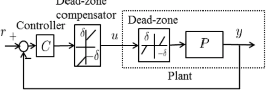
We consider a single-input and multi-output system which consists of a linear time- invariant part P and an input dead-zone D_δ as shown in Fig. 1. We assume that the

(4)

Figure 1: A system with an input dead-zone

Figure 2: Dead-zone compensation

input-output relation of the dead-zoneD_δ can be described as

D_δ(u) =





u−δ îf û^>δ 0 if |u| ≤δ u+δ îf û^<−δ

(1)

with a dead-zone interval[−δ^,δ^{] (}δ ^>0). As in [5], when we know the exact value of δ, we can eliminate the dead-zone nonlinearityD_δ by using its right inverse as

Dˆ_δ(u) =ˆ



 ˆ

u+δ ^if ^u^ˆ^>⁰ 0 if uˆ=0 ˆ

u−δ ^if ^u^ˆ^<⁰ ⁽²⁾

That is,D_δ◦Dˆ_δ =1, in other words,D_δ(Dˆ_δ(u)) =u. Hence, when we replace ˆD_δ in front ofD_δ as in Fig. 2, we can cancel the dead-zone.

In this paper, we consider a feedback control system to use ˆD_δ as depicted in Fig. 3.

In the control system, a feedback controllerC is designed to stabilizeP. In Fig. 3, r is the reference input, u is the control input, y is the measured output, respectively.

Unlike the ideal case where the exact value ofδ is available, it is difficult to cancel D_δ by ˆD_δ completely in practical application. The cancelation error causes the steady- state vibration in the control system whenPis unstable. Then, we need to determine an appropriate valueδ ^{in ˆ}^D_δ to suppress the steady-state periodic motion in the control system.

(5)

Figure 3: Configuration of a feedback control system with dead-zone compensation

3 Discrete-time Extremum Seeking Control For Peri- odic Steady-states

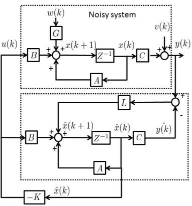
Extremum seeking control is known as a powerful adaptive method to optimize the control performance in real time. It is mainly used to optimize the control system with a constant steady-state output. In [6], an extremum seeking scheme for periodic steady- state outputs was proposed in the non-equilibrium case. In this thesis, we consider a discrete-time version of [6] which is summarized in Fig. 4. The configuration a feedback control system with a tuning parameterδ connected with discrete-time extremum seeking control as in Fig. 4. We consider a stabilized plant as

x(k+1) = f(x(k),δ^(k)) ⁽³⁾

y(k) = h(x(k)) (4)

The extremum seeking control aims to tune the parameterδ to minimize the cost function of performance output [6] by given as

J(δ^{(k)) =} [

1 N

∑k i=k−N

y(i)² ]¹

2

(5) whereNis the period of the steady-state outputy. The extremum seeking scheme uses a perturbation (dither) signal

d1(k) =acos2π

L k (6)

with the periodL∈Zand an estimate ˆδ of an optimal valueδ^∗by applying

δ^{(k) =}δ^ˆ^{(k) +}^d1(k) (7)

to the system. We denote the estimation error by

δ˜^{(k) =}δ^∗−δˆ^(k) ⁽⁸⁾

To use (7) and (8), we have

δ^{(k) =}δ^∗−δ˜^{(k) +}^d1(k). (9)

(6)

Figure 4: Discrete-time ESC scheme

This perturbed signal affects (5). By applying the Taylor series expansion to (5), we have

J(δ^{(k)) =} ^J(δ^∗−δ˜^{(k) +}^d1(k))

= J(δ^∗^{) +}∂^J

∂δ⁽δ^∗^)[(δ^∗−δ˜^{(k) +}^d1(k))−δ^∗^{] +}¹ 2

∂²^J

∂δ²^[(δ^∗−δ˜^{(k) +}^d1(k))−δ^∗^]²

∼= J(δ^∗^{) +}∂^J

∂δ⁽δ^∗^)(d²^(k)−δ˜^{(k) +}¹ 2

∂²^J

∂δ²⁽δ^∗^)(d²^(k)−δ˜^(k))²^, ⁽¹⁰⁾ whered₂(k)denotes the time delayed signal ofd₁(k)due to the dynamics in the closed-

loop system as

d₂(k) =acos2π

L (k−φ^), φ∈Z. (11)

SinceJ(δ⁾is optimal atδ^∗^,^∂_∂δ^J⁽δ^∗^{) =}^{0. Hence,} J(δ^(k))^∼⁼^J(δ^∗^{) +}¹

2

∂²^J

∂δ²⁽δ^∗^)(d2(k)−δ˜^(k))²^. ⁽¹²⁾ This cost function is multiplied by the demodulation signald₂(k), and applied into a moving-average filter, also called a mean-over-perturbation-period (MOPP) filter, over the period ofd2(k). Then, the output is

ξ^{(k) =} ¹ L

∑k j=k−L

d₂(j) (

J(δ^∗^{) +}¹ 2

∂²^J

∂δ²⁽δ^∗^)(d2(k)−δ˜^(k))² )

. (13)

By simple calculation, we have

∑k j=k−L

d2(j) =0,

∑k j=k−L

d₂²(j) = a²L 2 ,

∑k j=k−L

d³₂(j) =0. (14)

(7)

Hence, when we can assume that ˜δ⁽^j)is constant over the periodL, we have ξ^{(k) =}−a²

2

∂²^J

∂δ²⁽δ^∗⁾δ^˜^(k). ⁽¹⁵⁾ The signalξ^(k)is used to generate the estimate ˆδ by using the optimizer (the discrete- time integrator) as

δˆ^{(k) =}−K 1

z−1ξ^(k). ⁽¹⁶⁾

Herezis the time-shift operator, that iszδˆ^{(k) =}δ^ˆ^(k⁺1). Hence, (16) is equivalently δˆ^(k⁺^{1) =}δ^ˆ^(k)−Kξ^(k). ⁽¹⁷⁾ To use (7) and (13), we can rewrite (17) as

δ˜^(k⁺^{1) =} δ^˜^{(k) +}^Kξ^(k)

= (

1−Ka² 2

∂²^J

∂δ²⁽δ^∗⁾ )

δ˜^(k). ⁽¹⁸⁾

Hence, we have next theorem.

Theorem 1.

If

1−Ka² 2

∂²^J

∂δ²⁽δ^∗⁾ ^< ^1, ⁽¹⁹⁾ then an estimate ˆδ converges to the optimal valueδ^∗by extremum seeking. The convergence rate to the optimal value depends on the amplitudeaof the perturbation signal d₁andd₂, and the gainKof the optimizer. Since the Hessian ∂²^J

∂δ²⁽δ^∗⁾^of^Jis unknown, we should start with small values foraandKto find appropriate values. Moreover, the following underlying assumptions are also required [6], [14].

Assumption 1. For all fixed parameter δ over the range for tuning, the stabilized closed-loop system has a unique globally asymptotically stable steady-state solution with a constant period.

Assumption 2. The cost functionJ(δ⁾has a unique global minimum atδ^∗for steady- state performance.

4 Extremum Seeking Parameters Influence on Perfor- mance

The summarized of algorithm tuning dead-zone compensation by discrete-time extremum seeking which consist of

(8)

1. Design of a stabilizing controller for the closed-loop system,

2. Design of the cost function of the output measurement of the system,

3. Design parameters of extremum seeking such as frequency or period of perturbation or dither signal, MOPP filter, gain optimizer which check :

• Period of output y measured signal

• Output of the cost function signal with static or constant steady-state

• Assumption 1 and 2 are satisfied

• Convergence by Theorem 1

Futhermore, we can design and analyse how to choose properly parameters extremum seeking to tune dead-zone compensation for good performance and fast rejection dead- zone. The extent of the influence of parameters can be good performance if the parameters of extremum seeking are enlarged and reduced that will be further describe below.

• Gain of the optimizer K

Gain optimizerKconsider the convergence speed and stability system.

• Phase of the perturbation signalφ

In [6], phase of perturbation signal selects the constant φ ∈R≥0 which is an estimate of the sum of the time-varying delay of the plant dynamics and the performance measure of cost function for a good chosen.

• Period of perturbation L

Period of perturbation signal L should choose larger than period of cost function N. So, we check output signal of cost function before designing period of perturbation signal.

• Period of MOPP Filter L

Period of MOPP filter is same with the period of the perturbation signal.

• Amplitude of the perturbation signal a

For designing the amplitude of the perturbation signal, we select small value which is smaller than cost function value in initial parameter without extremum seeking.

5 Self-Balancing Robot

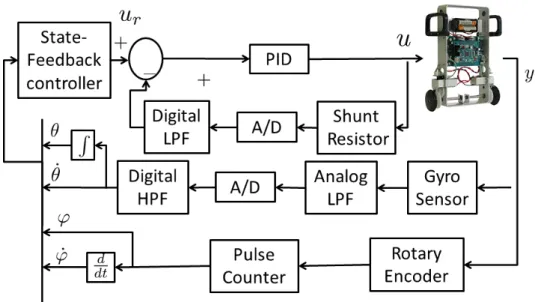
In this section, we use the discrete-time extremum seeking control discussed in the previous section to optimize a dead-zone compensation for self-balancing robot which is a commercial product called e-nuvo WHEEL shown in Fig. 5. The feedback controller Cfor the self-balancing robot is initially designed to use the model based on dynamic equations and the catalog parameters, and secondly done to use the model obtained by closed loop identification.

(9)

Figure 5: Modeling of the Self-balancing robot

6 Models of Self-Balancing Robot

6.1 Physical equation based model

As in [15], the state space continuous-time model of the self-balancing robotPin Fig. 5 can be derived from physical equations as

˙

x = A_cx+B_cu (20)

y = C_cx (21)

where x= [θ φ θ^˙ φ^˙^]^T consists of the angle of the body θ, the relative angle of the wheel to the bodyφ, the angular velocity of the body ˙θ and the relative angular velocity of the wheel to the body ˙φ. The control input u is electrical current. Together with Table 1 [15], [16], we haveA_c,B_cas

A_c =

[ 0₂_×₂ I₂_×₂

−E⁻¹G −E⁻¹F ]

=







0 0 1 0

0 0 0 1

104.05 0 0 0.06

−341.64 0 0 −0.37





,

B_c =

[ 0_2×2

−E⁻¹ζ ]

=





 0 0 37.8

−232.7





,

(22) where

E =

[ e11 e12

e₂₁ e₂₂ ]

+(

(M+m)r²_t +J_t) I₂,

F =

[ 0 c 0 0

]

, G=

[ 0 0

−mgl 0 ]

, ζ ⁼

[ η^{i K}t

0 ]

(23)

(10)

Table 1: Parameters of self-balancing robot

Mass of the cart (tire, draft shaft ,gear) [Kg] M 0.071

Mass of the body [Kg] m 0.5392

Moment of inertia of the body[Kg m²] J_p 2.160×10⁻³ Moment of inertia of the cart[Kg m²] J_t 8.632×10⁻⁵ Moment of inertia of motor rotor[Kg m²] J_m 1.30×10⁻⁷ Length between the wheel axle and gravity center of the body[m] l 0.1073

Radius of the wheel [m] r_t 0.02485

Friction of the wheel axle[Kg m²/ s] c 1×10⁻⁴ Torque constant of the motor [N m /A] K_t 2.79×10⁻³

Reduction ratio of the gear i 30

Efficiency drive system η ^0.75

e₁₁=e₂₂ =mlr_t+iJ_m e₁₂=i²J_m

e₂₁=2mlrt+ml²+Jp+Jm

(24) Since we measureφ^{and ˙}θ^,

C_c=

[ 0 1 0 0 0 0 1 0

] .

6.2 Closed-loop Identification Model

We obtain data measurement of the self-balancing robot commercial product e-nuvo WHEEL and identify data measurement. Identification experiment model is identification MOESP-type closed-loop subspace model identification (CL-MOESP) [17], [18].

The CL-MOESP identification model is dynamic model that is given by

A =







1.0033 −0.0298 0.0157 −0.0061 −0.0324 0.0079 0.9102 −0.2941 −0.0299 0.0013

−0.0030 0.1140 0.2547 −0.0970 0.0403

−0.0027 0.0123 −0.1012 1.0675 0.0177 0.0003 −0.0023 0.2437 0.0403 0.9341





,

B =







−1.2453 0.3671

−0.1786 0.0710

−0.0063





, D=

[ −0.0108 0.0401

] ,

C =

[ −0.0796 −0.2888 −0.0025 0.0075 −0.2407 0.0148 −0.2744 −0.8751 −0.1124 0.2605

]

(11)

Figure 6: Experiment e-nuvo WHEEL scheme

Dynamic model of self-balancing robot by identification is from data experiment e- nuvo WHEEL in Fig. 6 and used CL-MOESP identification in this research.

7 Design of a Stabilizing Controller

To discretize the continuous-time model (20) and (21) by zero-order hold, we obtain the discrete-time model

x(k+1) = A x(k) +B u(k) (25)

y(k) = C x(k) (26)

When we use the sampling periodT_s=0.01 sec, we have

A =







1 0 0.01 0

−0.02 1 −0.0001 0.01

1.04 0 1 0

−3.42 0 −0.02 1





,B=







0.002

−0.01 0.38

−2.32





,

C = Cc

The discrete-time model is used to design the discrete-time LQG controller [19], [20]

in Fig. 7 which minimizes E

[

τ→∞lim 1 τ

∑τ k=0

x^T(k)Qx(k) +u^T(k)Ru(k) ]

(27)

where Q and R are given constant weight matrices for whichQ=Q^T ≥0 ,R=R^T >0, under the existence of the process noise and the measurement noise. We assumed weight matrices Q=I₄,R= 1 and covariance of the process noiseW =1 and the

(12)

Figure 7: Discrete-time Linear Quadratic Gaussian scheme

measurement noiseV =0.012I₂ which means rms noise 1% on each sensor channel.

K is derived as

K= (B^TSB+R)⁻¹B^TSA, (28)

and the solutionS=S^T ≥0 of the associated Riccati equation

A^TSA−S−(A^TSB+N)(B^TSB+R)⁻¹(B^TSA+N^T) +Q=0 (29) The optimal L minimizingE[x(k)−x(k)]ˆ ^T[x(k)−x(k)]ˆ is given byL(k) =APC^T(CPC^T+ V)⁻¹ where P=P^T ≥0 is the unique positive-semidefinite solution of discrete al- gebraic Riccati equation. The discrete-time linear quadratic Gaussian (LQG) controller is given by connecting the discrete-time linear quadratic regulator (LQR) and the discrete-time Kalman filter according to block diagram in Fig. 7.

8 Physical-equation based Model

8.1 Dead-Zone Compensation

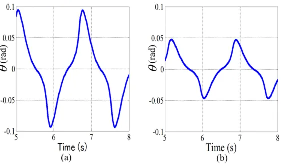
In the following, we set the actual dead-zone parameter δ ⁼2 as for the numerical simulations. When we do not use the dead-zone compensator (this corresponds to δˆ⁼^{0 in ˆ}D, the angle of the bodyθ shows periodic steady periodic steady-state motion with amplitude 0.1 rad (5.7 degree) as shown in Fig. 8 (a). On the other hand, when we use the dead-zone compensator ˆD_δ with ˆδ ⁼1, the amplitude of the periodic steady- state motion of the angle of the body θ is 0.05 rad (2.8 degree) as shown in Fig. 8

(13)

Figure 8: The angle of the bodyθ of the closed-loop system with dead-zoneD_δ(δ⁼²⁾ (a) with no dead-zone compensator, (b) with dead-zone compensator ˆD_δ(δˆ ⁼¹⁾ (b). Although the periodic steady-state motion is much reduced by the dead-zone compensator, it still remains due to the gap between the actualδ ^{and ˆ}δ in the dead- zone compensator. Hence, it is important to tune ˆδ to suppress the periodic steady-state motion completely.

8.2 Extremum Seeking for Tuning of Dead-Zone Parameter

For simplicity, we usey=θ for the output for extremum seeking control and the cost function

J(k) = [

1 N

∑k i=k−N

θ⁽ⁱ⁾² ]¹₂

whereas the output for feedback control isy= [φ θ^˙^]^T. The parameters for extremum seeking control are as follows; the amplitude and the period of the perturbation signal are a =1/16 and L =1800, the gain of the optimizer is K = 3, the time delay of the perturbation signal ind₂ isφ ⁼100, the period of cost function isN =180. The mean-over-perturbation-period can be implemented by a FIR filter. A simulation result where tuning dead-zone compensation by the discrete-time ESC starts att =200 sec is shown in Fig. 9 wherex[0] = [0.01 0 0 0]^T as the initial variable. The dead-zone compensation parameter ˆδ converges toδ⁼2.06 as shown in Fig. 9 (a). Although this final value is not the actual valueδ⁼2, the periodic steady-state motion in the bodyθ is sufficiently suppressed as shown in Fig. 9 (b). Indeed, the cost functionJ decreases to sufficiently small value as shown in Fig. 9 (c). This result shows that the small gap between the dead-zone parameter compensation and the actual one is acceptable.

(14)

Figure 9: A simulation result when extremum seeking is applied for tuning of dead- zone compensator. (a) the tuned value of dead-zone compensator, (b) the angle of the body, (c) the cost function

9 Simulation Results by CL-MOESP Identification Model

9.1 Dead-Zone Compensation

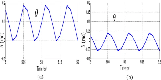
We applied the discrete-time LQG regulator to make stabilized unstabled plant from the CL-MOESP identification model of the Self-balancing robot because tuning by the discrete-time ESC was need stabilized plant. We utilized the discrete-time Kalman filter to estimation state and the discrete-time LQR to search state feedback gain. We used weight matricesQ=I₄,R=1 and covariance of process noiseW =1 and measurement noiseV =0.01²I₂which means rms noise 1% on each sensor channel. Then we set dead-zone parameterδ ⁼2 and the initial state as byx₀= [0.01 0 0 0]^T. So, we achieved simulation result of the CL-MOESP model of the closed-loop system without extremum seeking with dead-zone, dead-zone compensator and the discrete-time LQG regulator controller. When we utilize dead-zoneD_δ =2 and do not use the dead-zone compensator ˆD_δ=0, the angle of the bodyθ shows periodic steady-state motion with amplitude 0.2 (11.46 degree) rad as shown in Fig. 10 (a). When, we use the dead-zone

(15)

Figure 10: The angle of the body θ of CL-MOESP model of the closed-loop system with dead-zone D_δ(δ ⁼²⁾ (a) with no dead-zone compensator, (b) with dead-zone compensator ˆD_δ(δˆ ⁼¹⁾

compensator ˆD_δ with ˆδ ⁼1, the amplitude of the periodic steady-state motion of the angle of the bodyθ reduces to 0.05 rad (2.8 degree) as shown in Fig. 10 (b) for the CL-MOESP identification model.

9.2 Extremum Seeking for Tuning of Dead-Zone Parameter

We take the discrete-time ESC to tuning dead-zone compensation for rejecting vibration which is cost function from outputθ ^{by given}

J(δ^{) =} [

1 N

∑k i=k−N

θ⁽ⁱ⁾² ]¹₂

Afterward, we set extremum seeking parameters that are same with the previous setting of Self-balancing robot derived physical equations model. Simulation results of CL-MOESP model for tuning dead-zone compensation by the discrete-time ESC are shown in Fig. 11 withK=3 which are represented cost function of CL-MOESP model J in Fig. 11 (a) is decrease to minimum, the angle of the body of CL-MOESP model depict for rejection dead-zone and stabilized moving self-balancing robot in Fig. 11 (b), estimation dead-zone compensation ˆδ that is achieved 2 as fit as setting dead-zone it is shown in Fig. 11 (c) the tuned value of dead-zone compensator, but it needs time starting 200 second and achieved optimal value after 500 second forK=3. Afterthat, estimationξ Fig. 11 (d) is zero that indicate optimal performance.

10 Stability analysis

The stability of extremum seeking was first analyzed by Wang and Krsti`c [8]. They proposed averaging and singular perturbation to derive stability conditions of an ex-

(16)

Figure 11: Extremum seeking result when K =3 for CL-MOESP model. Time re- sponse of (a) cost function (b) the angle of the body (c) tuned parameter (d) estimated gradient of the cost function

tremum seeking feedback scheme [8] in which the averaging theorem adopted theorem 8.3 in Khalil as detail see [21] and Appendix C. To guarantee practical asymptotic stability, Teel et al. [22] proposed a generalized Lyapunov theorem.

Stability analysis of extremum seeking for periodic steady-state suggested by Har- ing et.al [6]. To apply extremum seeking, we used a stabilized controller which stabilize the plant of system which is a Discrete-Time Linear Quadratic Gaussian (LQG) controller to stabilize the closed-loop system. Stability of the closed loop system is ensured by appropriate state feedback gain and state estimation gain in LQG.

11 Conclusions

We are concluded the dissertation as follows:

• The dissertation proposed discrete-time extremum seeking control by moving average filter to tune input dead-zone compensation in real time and applied it to the stabilized self-balancing robot model with the dead-zone compensation.

• The effectiveness is illustrated by numerical simulations. In the simulations, the compensation parameter converges to the optimal value minimizing the cost function of the performance output.

• Stability analysis for non-linear system and discrete-time system, we used a stabilized controller which stabilize the plant of system.

(17)

12 Future Works

We will apply discrete-time extremum seeking control to eliminate dead-zone by experiment to e-nuvo WHEEL. However, it is not easy to apply in real time by experiment because the running of experiment e-nuvo WHEEL is quickly while the process of tuning dead-zone parameters by computer needs time also transfer data from computer to e-nuvo WHEEL has time-delay. Therefore, we will develop how to rapidly the process of tuning dead-zone parameters by extremum seeking. We will design programming of tuning by extremum seeking through micro-controller in e-nuvo WHEEL to control directly.

References

[1] G. Tao and P. V. Kokotovi´c, “Adaptive control of plants with unknown dead- zones,” Journal of IEEE Transactions on Automatic Control, vol. 39, no. 1, pp.

59–68, January, 1994.

[2] W. M. Bessa, M. S. Dutra, and E. Kreuzer, “An adaptive fuzzy dead-zone compensation scheme and its application to electro-hydraulic systems,”Journal of the Brazilian Society of Mechanical Scientist and Engineering, vol. XXXII, no. 1, pp.

1–7, January-March, 2010.

[3] ——, “Sliding mode control with adaptive fuzzy dead-zone compensation of an electro-hydraulic servo-system,” Journal of Intelligent and Robotic Systems, vol. 58, no. 1, pp. 3–16, May, 2009.

[4] J. O. Jang, H. T. Chung, and G. J. Jeon, “Saturation and deadzone compensation of systems using neural network and fuzzy logic,” inProceedings of The Ameri- can Control Conference, Potland, OR (USA), June 8-10, 2005, pp. 1715–1720.

[5] Y. Wakasa and K. Tanaka, “FRIT for Systems with Dead-Zone and Its Applica- tion to Ultrasonic Motors,” Journal of IEEJ Transactions on Electronics, Infor- mation and Systems, vol. 131, no. 6, pp. 1209–1216, 2011.

[6] M. Haring, N. V. de Wouw, and D. Neˇsi´c, “Extremum-seeking control for nonlinear systems with periodic steady-state outputs,”Automatica, vol. 49, no. 6, pp.

1883–1891, June 2013.

[7] K. Ariyur and M. Krsti´c, Real-time optimization by Extremum-seeking Control.

Wiley-Interscience, 2003.

[8] M. Krsti´c and H.-h. Wang, “Stability of extremum seeking feedback for general nonlinear dynamic systems ,”Automatica, vol. 36, pp. 595–601, 2000.

[9] Y. Tan, W. Moase, and C. Manzie, “Extremum seeking from 1922 to 2010,” in Proceedings of The 29th Chinese Control Conference, Beijing (China), December 10-13, 2010, pp. 14–26.

(18)

[10] J.-Y. Choi, M. Krsti´c, K. B. Ariyur, and J. S.Lee, “Extremum Seeking Control for Discrete-Time Systems,” Journal of IEEE Transactions on Automatic Control, vol. 47, no. 2, pp. 318–323, 2002.

[11] P. Frihauf, M. Krsti´c, and T. Bas, “Finite-Horizon LQ Control for Unknown Discrete-Time Linear Systems via Extremum Seeking,” in Proceedings of The 51st IEEE Conference on Decision and Control, Maui, Hawaii (USA), Decem- ber 10-13, 2012, pp. 5717–5722.

[12] K. B. Ariyur and M. Krsti´c, “Analysis and Design of Multivariable Extremum Seeking,” inProceedings of The American Control Conference, Anchorage, AK, May 8-10, 2002, pp. 2903–2908.

[13] M. Haring, “Extremum-seeking control for steady-state performance optimization of nonlinear plants with periodic steady-state outputs,” Ph.D. dissertation, Eindhoven University of Technology, June, 2011.

[14] B. Hunnekens, M. Haring, N. V. D. Wouw, and H. Nijmeijer, “Steady-state performance optimization for variable-gain motion control using extremum seeking,” in Proceedings of The 51st IEEE Conference on Decision and Control (CDC), Maui, Hawaii (USA), December, 10-13, 2012, pp. 3796–3801.

[15] ZMP, Stabilization and Control stable running of the Wheeled Inverted Pendulum Development of Educational Wheeled Inverted Robot e-nuvo WHEEL ver. 1.0. ZMP INC, (in Japanese). [Online]. Available: {http:

//www.zmp.co.jp/e-nuvo/pdf/wheel/wheel paper.pdf}

[16] ——,Manual Designing control system Robot e-nuvo WHEEL ver. 1.0.0”. ZMP INC, (in Japanese), 2007.

[17] H.Oku, “Identification experiment of a cart system using closed-loop subspace model identification methods,” in Proceedings of SICE Annu. Conf. on Control Systems,(in Japanese), 2008.

[18] ——, “On asymptotic properties of moesp-type closed-loop subspace model identification,” in Proceedings of the 19th International Symposium on Mathe- matical Theory of Networks and Systems, Budapest, Hungary, July 5-9, 2010, pp.

1015–1022.

[19] J. F. Franklin, J. D. Powell and M. L. Workman, Digital Control of Dynamic Systems, 3rd ed. Addison Wesley Longman, Inc, 1998.

[20] S. Skogestad and I. Postlethwaite,Multivariable Feedback Control Analysis and design, 2nd ed. John Wiley and Sons, 2001.

[21] H. K.Khalil,Nonlinear Systems, 1st ed. Macmillan Publishing Company, 1992.

[22] A. R. Teel, J. Peuteman, and D. Aeyels, “Semi-global practical asymptotic stability and averaging,”Journal of Systems and Control Letters, vol. 37, pp. 329–334, May, 1999.

(19)