Star Formation 1

Star Formation ¹

Kohji Tomisaka

National Astronomical Observatory Japan May 8, 2007

1

http://yso.mtk.nao.ac.jp/˜tomisaka/Lecture Notes/StarFormation/3.pdf

Copyright c °2001-2004 by Tomisaka, K.

version 0.5: August 5, 2001

version 1.0: August 30, 2001

version 2.0: November 8, 2003

version 3.0: June 1, 2004

Contents

1 Introduction 1

1.1 Interstellar Matter . . . . 1

1.2 Case Study — Taurus Molecular Clouds . . . . 2

1.3 T Tauri Stars . . . . 4

1.4 Spectral Energy Distribution (SED) . . . . 6

1.5 Protostars . . . . 8

1.5.1 B335 . . . . 8

1.5.2 L1551 IRS 5 . . . . 12

1.6 L 1544: Pre-protostellar Cores . . . . 15

1.7 Magnetic Fields . . . . 15

1.7.1 Prestellar Core . . . . 15

1.7.2 Cores with Protostars . . . . 17

1.8 Density Distribution . . . . 22

1.9 Mass Spectrum . . . . 25

1.10 Line Width - Size Relation . . . . 27

2 Physical Background 29 2.1 Basic Equations of Hydrodynamics . . . . 29

2.2 The Poisson Equation of the Self-Gravity . . . . 29

2.3 Free-fall Time . . . . 30

2.3.1 Accretion Rate . . . . 32

2.4 Gravitational Instability . . . . 33

2.4.1 Linear Analysis . . . . 33

2.4.2 Sound Wave . . . . 34

2.5 Jeans Instability . . . . 35

2.6 Gravitational Instability of Thin Disk . . . . 36

2.6.1 Rotating Disk . . . . 38

2.7 Convective Instability . . . . 39

2.8 Super- and Subsonic Flow . . . . 40

2.8.1 Flow in the Laval Nozzle . . . . 40

2.8.2 Steady State Flow under an Influence of External Fields . . . . 41

2.8.3 Stellar Wind — Parker Wind Theory . . . . 43

2.9 Virial Analysis . . . . 46

2.10 Radiative Transfer . . . . 48

2.10.1 Radiative Transfer Equation . . . . 48

2.10.2 Einstein’s Coefficients . . . . 50

i

ii CONTENTS

2.10.3 Relation of Einstein’s Coefficients to Absorption and Emissivity . . . . 51

3 Galactic Scale Star Formation 53 3.1 Schmidt Law . . . . 53

3.1.1 Global Star Formation . . . . 53

3.1.2 Local Star Formation Rate . . . . 54

3.2 Gravitational Instability of Rotating Thin Disk . . . . 55

3.2.1 Tightly Wound Spirals . . . . 57

3.2.2 Toomre’s Q Value . . . . 58

3.3 Spiral Structure . . . . 59

3.4 Density Wave Theory . . . . 60

3.4.1 Group Velocity . . . . 62

3.5 Galactic Shock . . . . 63

4 Local Star Formation Process 69 4.1 Hydrostatic Balance . . . . 69

4.1.1 Bonnor-Ebert Mass . . . . 70

4.1.2 Equilibria of Cylindrical Cloud . . . . 71

4.2 Virial Analysis . . . . 72

4.2.1 Magnatohydrostatic Clouds . . . . 73

4.3 Subcritical Cloud vs Supercritical Cloud . . . . 75

4.4 Ambipolar Diffusion . . . . 75

4.4.1 Ionization Rate . . . . 75

4.4.2 Ambipolar Diffusion . . . . 76

4.5 Dynamical Collapse . . . . 79

4.5.1 Inside-out Collapse Solution . . . . 81

4.5.2 Protostellar Evolution of Supercritical Clouds . . . . 84

4.6 Accretion Rate . . . . 85

4.7 Outflow . . . . 87

4.7.1 Magneto-driven Model . . . . 87

4.7.2 Entrainment Model . . . . 91

4.8 Evolution to Star . . . . 91

4.9 Example of Numerical Simulation . . . . 94

4.10 Evolution in the H-R diagram . . . . 97

4.10.1 Main Accretion Phase . . . . 97

4.10.2 Premain-sequence Evolution . . . 102

Bibliography 105 A Basic Equation of Fluid Dynamics 111 A.1 What is fluid? . . . 111

A.2 Equation of Motion . . . 111

A.3 Lagrangian and Euler Equations . . . 112

A.4 Continuity Equation . . . 113

A.4.1 Expression for Momentum Density . . . 113

A.5 Energy Equation . . . 114

A.5.1 Polytropic Relation . . . 114

A.5.2 Energy Equation from the First Law of Theromodynamics . . . 115

CONTENTS iii

A.6 Shock Wave . . . 115

A.6.1 Rankine-Hugoniot Relation . . . 115

B Basic Equations of Magnetohydrodynamics 117 B.1 Magnetohydrodynamics . . . 117

B.1.1 Flux Freezing . . . 117

B.1.2 Basic Equations of Ideal MHD . . . 118

B.1.3 Axisymmetric Case . . . 118

C Hydrostatic Equilibrium 121 C.1 Polytrope . . . 121

C.2 Magnetohydrostatic Configuration . . . 123

D Basic Equations for Radiative Hydrodynamics 125 D.1 Radiative Hydrodynamics . . . 125

E Random Velocity 127

Chapter 1

Introduction

1.1 Interstellar Matter

"Coronal" Gas

HII Regions

Diffuse Cloud

Globule Molecular Cloud

log n (cm-3) 0.0

lo g T (K)

-4.0 -2.0 2.0 4.0 6.0 8.0 10.0 12.0 14.0 16.0 18.0 20.0 22.0 0.0

1.0 2.0 3.0 4.0 5.0 6.0 7.0 8.0

Warm or Hot Core

Mass Loss from Red Giant Interaction with Supernova

Photo-dissociation

Supernova

Intercloud Gas

First Stellar Core

Quasi-static Contraction

Second Collapse

Dissociation of H

Second Stellar Core Star

Figure 1.1: Multiphases of the interstellar medium. The temperature and number density of gaseous objects of the interstellar medium in our Galaxy are summarized. Originally made by Myers (1978), reconstructed by Saigo (2000).

Figure 1.1 shows the temperature and number density of gaseous objects in our Galaxy. Cold interstellar medium forms molecular clouds (T ∼ 10K) and diffuse clouds (T ∼ 100K). Warm inter- stellar medium 10

K < ∼ T < ∼ 10

K are thought to be pervasive (wide-spread). HII regions are ionized by the Ly continuum photons from the nearby early-type stars. There are coronal (hot but tenuous) gases with T ∼ 10

K in the Galaxy, which are heated by the shock fronts of supernova remnants.

Pressures of these gases are in the range of 10

K cm

< ∼ p< ∼ 10

K cm

, except for the HII regions.

This may suggest that gases are in the pressure equilibrium.

1

2 CHAPTER 1. INTRODUCTION In this figure, a theoretical path from the molecular cloud core to the star is also shown. We will see the evolution more closely in Chapter 4.

Globally, the molecular form of Hydrogen H

is much abundant inside the Solar circle, while the atomic hydrogen HI is more abundant than molecular H

in the outer Galaxy. In Figure 1.2 (left), the radial distributions of molecular and atomic gases are shown. The right panel shows similar distributions for four typical external galaxies (M51, M101, NGC6946, and IC342). This indicates these distributions are similar with each other. HI is distributed uniformly, while H

density increases greatly reaching the galaxy center. In other words, only in the region where the total (HI+H

) density exceeds some critical value, H

molecules are distributed.

Figure 1.2: Radial distribution of H

(solid line) and HI (dashed line) gas density. (Left:) our Galaxy.

Converting from CO antenna temperature to H

column deity, n(CO)/n(H

) = 6 × 10

is assumed.

Taken from Gordon & Burton (1976). (Right:) Radial distribution of H

and HI gas for external galaxies. The conversion factor is assumed constant X(H

/CO) = 3 × 10

H

/K km s

. Taken from Honma et al (1995).

1.2 Case Study — Taurus Molecular Clouds

Figure 1.3 (left) shows the

CO total column density map of the Taurus molecular cloud (Mizuno et

al 1995) whose distance is 140 pc far from the Sun. Since

CO contains

C, a rare isotope of C, the

abundance of

CO is much smaller than that of

CO. Owing to the low abundance, the emission

lines of

CO are relatively optically thiner than that of

CO. Using

CO line, we can see deep

inside of the molecular cloud. The distributions of T Tauri stars and

CO column density coincide

with each other. Since T Tauri stars are young pre-main-sequence stars with M ∼ 1M

, which are in

the Kelvin-Helmholtz contraction stage and do not reach the main-sequence Hydrogen burning stage,

it is shown that stars are newly formed in molecular clouds.

1.2. CASE STUDY — TAURUS MOLECULAR CLOUDS 3

Figure 1.3: (Left)

CO total column density map of the Taurus molecular cloud (Mizuno et al 1995).

Taken from their home page with URL of http://www.a.phys.nagoya-u.ac.jp/nanten/taurus.html (in Japanese). T Tauri stars, which are thought to be pre-main-sequence stars in the Kelvin-Helmholtz contraction stage, are indicated by bright spots. (Right) C

O map of Heiles cloud 2 region in the Taurus molecular cloud (Onishi et al. 1996). This shows clearly that the cloud is composed of a number of high-density regions.

Since

O is much more rare isotope (

O/

O ¿

C/

C), the distribution of much higher- density gases is explored using C

O lines. Figure 1.3 (right) shows C

O map of Heiles cloud 2 in the Taurus molecular cloud by Onishi et al (1996). This shows us that there are many molecular cloud cores which have much higher density than the average. Many of these molecular cloud cores are associated with IRAS sources and T Tauri stars. It is shown that star formation occurs in the molecular cloud cores in the molecular cloud. They found 40 such cores in the Taurus molecular cloud.

Typical size of the core is ∼ 0.1 pc and the average density of the core is as large as ∼ 10

cm

. The mass of the C

O cores is estimated as ∼ 1 − 80M

.

H

CO

ions are excited only after the density is much higher than the density at which CO molecules are excited. H

CO

ions are used to explore the region with higher density than that observed by C

O. Figure 1.4 shows the map of cores observed by H

CO

ions. The cores shown in the lower panels are accompanied with infrared sources. The energy source of the stellar IR radiation is thought to be maintained by the accretion energy. That is, since the gravitational potential energy at the surface of a protostar with a radius R

and a mass M

is equal to Φ ' −GM

/R

, the kinetic energy of the gas accreting on the stellar surface is approximately equal to ∼ GM

/R

. The energy inflow rate owing to the accretion is (∼ GM

/R

) × M ˙ ∼ (GM

/R

) × A(c

/G), where ˙ M = A(c

/G) is the mass accretion rate. In the upper panels, the cores without IR sources are shown. This core does not show accretion but collapse. That is, before a protostar is formed, the core itself contract owing to the gravity, which is explained closely in chapter 4.

In Figure 1.4, H

CO

total column density maps of the C

O cores are shown. Cores in the lower panels have associated IRAS sources, while the cores in the upper panels have no IRAS sources.

Since the IRAS sources are thought to be protostars or objects in later stage, the core seems to evolve from that without an IRAS sources to that with an IRAS source. From this, the core with an IRAS source is called protostellar core, which means that the cores contain protostars. On the other hand, the core without IRAS source is called pre-protostellar core or, in short, pre-stellar core.

Figure 1.4 shows that the prestellar cores are less dense and more extended than the protostellar

core. This seems to suggest the density distribution around the density peak changes between before

4 CHAPTER 1. INTRODUCTION

Figure 1.4: Pre-protostellar vs protostellar cores (H

CO

map). Upper panel shows the C

O cores without associated IRAS sources. Lower panel shows the cores with IRAS sources. Taken from Fig.1 of Mizuno et al. (1994)

and after the protostar formation.

1.3 T Tauri Stars

T Tauri stars are observationally late-type stars with strong emission lines and irregular light varia- tions associated with dark or bright nebulosities. T Tauri stars are thought to be low-mass pre-main- sequence stars, which are younger than the main-sequence stars. Since these stars are connecting between protostars and main-sequence stars, they attract attention today. More massive counter- parts are called Herbig Ae-Be stars. They are doing the Kelvin-Helmholtz contraction in which the own gravitational energies released as it contracts gradually and this is the energy source of the lumi- nosity. Many emission lines are found in the spectra of T Tauri stars. WTTS (Weak emission T Tauri Stars or Weak line T Tauri Stars) and CTTS (Classical T Tauri Stars) are classified by their equiva- lent widths (EWs) of emission lines. That is, the objects with an EW of Hα emission < 1nm = 10˚ A is usually termed a WTTS. Figure 1.5 is the HR diagram (T

−L

) of T Tauri stars in Taurus-Auriga region (Kenyon & Hartman 1995). WTTSs distribute near the main-sequence and CTTSs are found even far from the main-sequence. A number of theoretical evolutional tracks for pre-main-sequence stars with M ∼ 0.1M

− 2.5M

are shown in a solid line, while the isochorones for ages of 10

yr, 10

yr, and 10

yr are plotted in a dashed line. Vertical evolutional paths are the Hayashi convective track. Since D=

H has a much lower critical temperature (and density) for a fusion nuclear reaction to make He than

H, Deuterium begins to burn before reaching the zero-age-main sequence. This occurs near the isochrone for the age of 10

yr and some activities related to the ignition of Deuterium seem to make the central star visible (Stahler 1983).

Disk Frequency

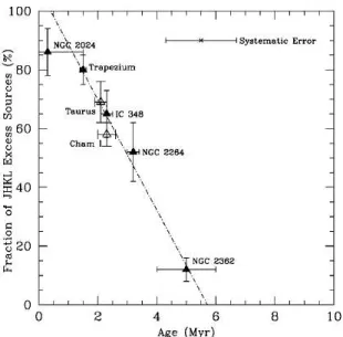
Infrared studies of T Tauri stars in star-forming regions have suggected that initial disk frequency if rather high and that the disk lifetimes are relatively short 3 − 15Myr. From JHKL photometry, Haish, Lada, & Lada (2001) obtained the fraction of disk-bearing stars for 6 star firmation regions.

L band excess emission indicates an accompanied disk. The fraction is a decreasing function of age

1.3. T TAURI STARS 5

Figure 1.5: HR diagram of T Tauri stars. Many emission lines are found in the spectra of T Tauri

stars. WTTS (Weak Emission T Tauri Stars) and CTTS (Classical T Tauri Stars) are classified by

the equivalent widths of emission lines. That is, the objects with an EW of Hα emission < 1nm is

usually termed a WTTS. Taken from Fig.1.2 of Hartmann (1998).

6 CHAPTER 1. INTRODUCTION

Figure 1.6: Fractions of IR excess sources in respective clusters are plotted againt the age of the clusters.

of the cluster as in Figure 1.6. This figure shows clearly that the disk fraction is initially very high ( > ∼ 80%) and rapidly decreases with increasing cluster age. In 3 Myr a half of the disk stars lose their disks. Overall disk lifetime is estimated as ∼ 6Myr.

1.4 Spectral Energy Distribution (SED)

A tool to know the process of star formation is provided by the spectral energy distribution (SED) mainly in the near- and mid-infrared light. T Tauri stars and protostars have typical respective SEDs.

IR SEDs of T Tauri stars were classified into three as Class I, Class II, and Class III, from a stand- point of relative importance of the radiation from a dust disk to the stellar black-body radiation.

Today, the classification is extended to the protostars, which is precedence of the T Tauri stars, and they are called Class 0 objects. (Unfortunately, there is no zero in Roman numerals.) In Figure 1.7, typical SEDs and models of emission regions are shown.

1. Class III is well fitted by a black-body spectrum, which shows the energy mainly comes from a central star. This SED is observed in the weak-line T Tauri stars. Although T Tauri stars show emission lines of such as the Hydrogen Balmar sequence, the weak-line T Tauri stars do not show prominent emission lines, which indicates the amount of gas just outside the star (this seems to be supplied by the accretion process) is small. In this stage, a disk has been disappeared or an extremely less-massive disk is still alive.

2. Class II SED is fitted by a single-temperature black-body plus excess IR emission. This shows

that there is a dust disk around a pre-main sequence star and it is heated by the radiation

from a central star. The width of the spectrum of the disk component is much wider than that

expected from a single-temperature black-body radiation. Thus, the disk has a temperature

gradient which decreases with increasing the distance from the central star. In this stage, the

dust disk is more massive than that of Class III sources. Classical T Tauri stars have such

SEDs.

1.4. SPECTRAL ENERGY DISTRIBUTION (SED) 7

Figure 1.7: Spectral Energy Distribution (SED) of young stellar objects (YSOs) and their models.

(Left:) ν − νF

plot taken from Lada (1999). (Right:) λ − λF

plot taken from Andr´e (1994)

3. In Class I SED, the mid infrared radiation which seems to come from the dust envelope is predominant over the stellar black-body radiation. Since the stellar black-body radiation seems to escape at least partially from the dust envelope, a relatively large solid angle is expected for a region where the dust envelope does not intervene.

4. Class 0 SED seems to be emitted by an isothermal dust with ∼ 30K. The protostar seems to be completely covered by gas and dust and is obscured with a large optical depth by the dust envelope. No contribution can be reached from the stellar-black body radiation.

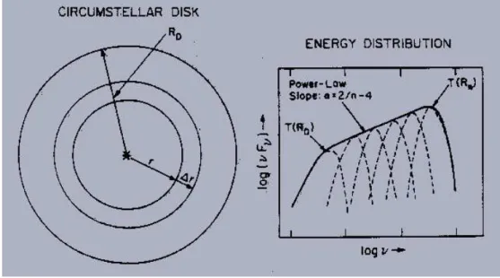
The reason why the emission from the disk becomes wide in the spectral range is understood (Fig.1.8) as follows: Temperature of the disk is determined by a balance of heating and cooling.

Assuming the disk is geometrically thin but optically thick, the cooling per unit area is given by

the equation of the black-body Planck radiation. Therefore, the temperature is determined by the

heating predominantly by viscous heating and extra heating by the radiation from the central star.

8 CHAPTER 1. INTRODUCTION

Figure 1.8: Explanation for the spectral index of the emission from a geometrically thin but optically thick disk. Taken from Fig.16 of Lada (1999).

The flux density emitted by the disk is given by νF

∼

Z

νπB

[T (r)]2πrdr ∼ r(T or ν)

νB

. (1.1) Assuming the radial distribution of temperature as

T = T

µ R

R

¶

, (1.2)

(q = 3/4 for the standard accretion disk) and taking notice that each temperature in the disk radiates at a characteristic frequency ν ∝ T (the Wien’s law for black-body radiation)

νF

∼ r

νB

∝ ν

T

∝ ν

, (1.3)

where we used the fact that the peak value of B

∝ ν

. Therefore, it is shown that νF

∝ ν

; n = 4 − 2

q . (1.4)

As shown in the previous section, we have no young stellar objects found by IR before a protostar is formed. These kind of objects (pre-protostellar core) are often called Class −1. The classification was originally based on the SED and did not exactly mean an evolution sequence. However, today YSOs are considered to evolve as the sequence of the classes: Class −1 → Class 0 → Class I → Class II → Class III → main-sequence star.

1.5 Protostars

1.5.1 B335

B335 is a dark cloud (Fig.1.9) with a distance of D ' 250pc. Inside the dark cloud, a Class 0 IR

source is found. The object is famous for the discovery of gas infall motion. In Figure 1.10, the

1.5. PROTOSTARS 9

Figure 1.9: Near infrared images of B335, which is Class 0 source.

Figure 1.10: Line profile of CS J = 2 − 1 line radio emission. Model spectra illustrated in a dashed

line (Zhou 1995) are overlaid on to the observed spectra in a solid line (Zhoug et al 1993).

10 CHAPTER 1. INTRODUCTION

Figure 1.11: Explanation of blue-red asymmetry when we observe a spherical symmetric inflow mo- tion. An isovelocity curve for the red-shifted gas is plotted in a solid line. That for the blue-shifted gas is plotted in a dashed line. Taken from Fig.14 of Lada (1999).

line profiles of CS J = 2 − 1 line emissions are shown (Zhou et al. 1993). The relative position of the profiles correspond to the position of the beam. (9,9) represents the offset of (9”,9”) from the center. At the center (0,0), the spectrum shows two peaks and the blue-shifted peak is brighter than the red-shifted one. This is believed to be a sign of gas infall motion. The blue-red asymmetry is explained as follows:

1. Considering a spherical symmetric inflow of gas, whose inflow velocity v

increases with reaching the center (a decreasing function of r)

2. Considering a gas element at r moving at a speed of v

(r) < 0, the velocity projected on a line-of-sight is equal to

v

= v

+ v

cos θ, (1.5)

where v

represents the systemic velocity of the cloud (line-of-sight velocity of the cloud center) and θ is the angle between the line-of-sight and the position vector of the gas element.

The isovector lines, the line which connect the positions whose procession/recession velocities are the same, become like an ellipse shown in Fig.1.11.

3. An isovelocity curve for the red-shifted gas is plotted in a solid line. That for the blue-shifted gas is plotted in a dashed line. If the gas is optically thin, the blue-shifted and red-shifted gases contribute equally to the observed spectrum and the blue- and red-shifted peaks of the emission line should be the same.

4. In the case that the gas has a finite optical depth, for the red-shifted emission line a cold gas in

the fore side absorbs effectively the emission coming from the hot interior. On the other hand,

for the blue-shifted emission line, the emission made by the hot interior gas escapes from the

cloud without absorbed by the cold gas (there is no cold blue-shifted gas).

1.5. PROTOSTARS 11

Figure 1.12: C

O total column density map (left) and H

CO

channel map (right) of B335 along with the position-velocity maps along the major and minor axes. Taken from Fig.3 of Saito et al (1999).

5. As a result, the blue peak of the emission line becomes more prominent than that of the read- shifted emission. This is the explanation of the blue-red asymmetry.

In Figure 1.10, model spectra calculated with the Sobolev approximation (Zhou 1995) are shown.

These show the blue-red asymmetry (the blue line > the red line).

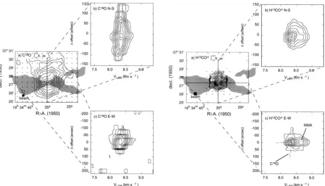
Early observation of star forming regions have revieled fast molecular outflow are often ejected from the central protostar with > ∼ 10km s

. B335 is also a typical outflow source. In Figure 1.12, distributions of high density gases traced by the C

O and H

CO

lines are shown as well as the bipolar outflow whose outline is indicated by a shadow (Hirano et al 1988). Comparing left and right panels, it is shown that the distribution of C

O gas is more extended than that of H

CO

which traces higher-density gas. And the distribution of the H

CO

is more compact and the projected surface density seems to show the the actual distribution is spherical. And the molecular outflow seems to be ejected in the direction of the minor axis of the high-density gas. It may suggest that (1) a molecular outflow is focused or collimated by the effect of density distribution or that (2) collimation is made by the magnetic fields which run preferentially perpendicularly to the gas disk. This gas disk is observed by these high density tracers.

Combining the C

O and H

CO

distributions, the surface density distribution along the major axis is obtained by Saito et al (1999). From the lower panel of Figure 1.13, the column density distribution is well fitted in the range from 7,000 to 42,000 AU in radius,

Σ(r) = 6.3 × 10

cm

µ r

10

AU

¶

, (1.6)

where they omitted the data of r< ∼ 7000 since the beam size is not negligible. Similar power-law

density distributions are found by the far IR thermal dust emission.

12 CHAPTER 1. INTRODUCTION

Figure 1.13: Column density distribution N

(r) derived from the H

CO

and C

O data taken by the Nobeyama 45 m telescope. Taken from Fig.9 of Saito et al (1999).

1.5.2 L1551 IRS 5

Figure 1.14: (Left:)

CO column density distribution. The contour lines represent the distribution of

CO column density. 2.2 µm infra-red reflection nebula is shown in grey scale which was observed by Hoddap (1994). (Right:) Schematic view of L1551 IRS5 region.

L1551 IRS 5 is one of the most well studied protostellar objects. This has an infra-red emission

nebulosity (Fig.1.14). It is believed that there is a hole perpendicular to the high-density disk and the

emission from the central star escapes through the hole and irradiate the nebulosity. In this sense this

is a reflection nebula. L1551 IRS 5 has an elongated structure of dense gas similar to that observed

in B335. The gas is extending in the direction from north-west to south-east [Fig.1.14 (left)]. Since

the opposite side of the nebulosity is not observed, the opposite side of nebulosity seems to be located

beyond the high-density disk and be obscured by the disk. This is possible if we see the south surface

of the high-density disk as in Figure 1.14 (right).

1.5. PROTOSTARS 13

Figure 1.15: Isovelocity contours measured by the

CO J = 1 − 0 line. It should be noticed that the isovelocity lines run parallelly to the major axis. The north-eastern side shows a red-shift and the south-western side shows a blue-shift.

Infall Motion

The inflow motion is measured. Figure 1.15 shows the isovelocity contours measured by the

CO J = 1 −0 observation (Ohashi et al 1996). It should be noticed that the isovelocity lines run parallelly to the major axis. The north-eastern side shows a red-shift and the south-western side shows a blue- shift. Considering the configuration of the gas disk shown in Fig.1.14 (right), this pattern of isovelocity contours indicates not outflow but inflow. That is, the north-east side is a near side of the disk and the south-west side is a far side. Since a red-shifted motion is observed in the near side and a blue-shifted motion is observed in the far side, it should be concluded that the gas disk of the L1551 IRS5 is now infalling.

Optical Jet

HST found two optical jets emanating from L1551 IRS5. This has been observed by SUBARU telescope, which found jet emission is dominated by [FeII] lines in the J- and H-bands. The jet extents to the south-western direction and disappears at ∼ 10” ' 1400AU from the IRS5. The width-to-length ratio is very small < ∼ 1/10 or less, while the bipolar molecular outflow shows a less collimated flow. As for the origin of the two jets, these two jets might be ejected from a single source.

However, since there are at least two radio continuum sources in IRS5 within the mutual separation

of ∼ 0.”5 [see Fig.1.16 (right)], these jets seem to be ejected from the two sources independently.

14 CHAPTER 1. INTRODUCTION

Figure 1.16: (Left:) Infrared image (J- and K-band) of the IR reflection nebula around L1551 IRS5

by SUBARU telescope. Taken from Fig.1 of Itoh et al. (2000). (A jpeg file is available from the

following url: http://SubaruTelescope.org/Science/press release/9908/L1551.jpg). (Right:)

Central 100 AU region map of L1551 IRS5. This is taken by the λ = 2.7cm radio continuum

observation. Deconvolved map (lower-left) shows clearly that IRS5 consists of two sources. Taken

from Looney et al. (1997).

1.6. L 1544: PRE-PROTOSTELLAR CORES 15 Although the lengths of these jets are restricted to 10”, Herbig-Haro jets, which are much larger than the jets in L1551 IRS5, have been found. HH30 has a ∼ 500 AU-scale jet whose emission is mainly from the shock-excited emission lines. One of the largest ones is HH111, which is a member of the Orion star forming region and whose distance is as large as D ∼ 400pc, and a jet with a length of

∼ 4pc is observed. Source of HH111 system is thought to consist of at least binary stars or possibly triple stars [Reipurth et al (1999)]. Star A, which coincides with a λ = 3.6 cm radio continuum source (VLA 1), shows an elongation in the VLA map whose direction is parallel to the axis of the jet. Therefore, star A is considered to be a source of the jet. Since the VLA map of star A shows another elongated structure perpendicular to the jet axis, star A may be a binary composed by two outflow sources.

1.6 L 1544: Pre-protostellar Cores

L1544 is known as a pre-protostellar core (Taffala et al 1998). That shows an infall motion but this contains no IR protostars. In Figure 1.18(left), CCS total column density map is shown, which shows an elongated structure. Ohashi et al (1999) have found both rotation and infall motion in the cloud.

Position-velocity (PV) diagram along the minor axis shows the infall motion. That along the major axis indicates a rotational motion, which is shown by a velocity gradient. Due to a finite size of the beam, a contraction motion is also shown in the PV diagram along the major axis.

1.7 Magnetic Fields

Directions of magnetic field are studied by (1) measuring the polarization of light which is suffered from interstellar absorption. In this case the direction of magnetic field is parallel to the polarization vector. The reason is explained in Figure 1.19. In the magnetic fields, the dusts are aligned in a way that their major axes are perpendicular to the magnetic field lines. Such aligned dusts absorb selectively the radiation whose E-vector is parallel to their major axes. As a result, the detected light has a polarization parallel to the magnetic field lines.

However, the polarization measurement in the near IR wavelength limited to the region with low gas density, because background stars suffer severe absorption and becomes hard to be observed if we want to measure the polarization of the high-density region. More direct method is (2) the measurement of the linear polarization of the thermal emission from dusts in the mm (or sub-mm) wavelengths; in this case the direction of magnetic field is perpendicular to the polarization vector.

The mechanism is explained in Figure 1.19b. The aligned dusts, whose major axes are perpendicular to the magnetic field lines, emit the radiation whose E-vector is parallel to the major axes. Since the absorption does not have a severe effect in this mm wavelengths, this gives information the magnetic fields deep inside the clouds.

1.7.1 Prestellar Core

Figure 1.20 illustrates the polarization maps of three prestellar cores (L1544, L183, and L43) done

in the 850 µm band by JCMT-SCUBA. In L1544 and L183 the mean magnetic fields are at an angle

of 30 deg to the minor axes of the cores. L43 is not a simple object; there is a T Tauri star located

in the second core which extends to south-western side of the core (an edge of this core is seen near

the western SCUBA frame boundary). And a molecular outflow from the source seems to affect

the core. The magnetic field as well as the gas are swept by the molecular outflow. L43 seems an

exception. The fact that the mean magnetic fields are parallel to the minor axis of the high-density

16 CHAPTER 1. INTRODUCTION

Figure 1.17: A mosaic image of HH 111 based on HST NICMOS images (bottom) and WFPC2 images

(top). Taken from Fig.1 of Reipurth et al (1999).

1.7. MAGNETIC FIELDS 17

Figure 1.18: CCS image of prestellar core L1544. (Left:) Total intensity map. (Right:) PV diagrams along the minor axis (left) and along the major axis (right).

gas distribution seems to mean gas contracts preferentially in the direction parallel to the magnetic fields.

1.7.2 Cores with Protostars

Bok Globules

Bok globules are isolated dark clouds. Wolf, Launhardt & Henning (2003) have studied the relation between the magnetic field and outflow directions. Figure 1.21 displays the direction of the magnetic field obtained with JCMT-SCUBA polarization observation in 850µm as well as the outflow found by 13CO observation of Chandler & Sargent (1993) and

CO observation by Yun & Clemens (1994).

In B 335, CB 230 and CB 244 outflows are oriented in the direction perpendicular to the major axis of the globules. The magnetic field is running parallel to the outflow but perpendicular to the major axis. This means that a disk is formed with a gas flowing along the magnetic field. Further, the outflow is generated by a twisted magnetic field which is an outcome of a rotating disk. In globule CB 54, the alignment is not perfect, that is, magnetic field direction is slightly aligned with the outflow (Wolf, Launhardt & Henning 2003). This seems to stengthen the magnetic origin of the outflow and magnetically guided disk formation.

It is clearly shown that the polarization anti-correlates with the intensity of the thermal emission.

This might be due to the observational error in the low intensity region (or low S/N region). This

may be related to physical processes such as (1) the alingnment owing to the magnetic field becomes

inefficient in high density region or (2) the magnetic field is tangled in the dense region and the

polarization due to the aligned dust is canceled.

18 CHAPTER 1. INTRODUCTION

Figure 1.19: Explanation how the polarized radiation forms. Taken from Weintraub et al.(2000).

1.7. MAGNETIC FIELDS 19

Figure 1.20: Directions of B-Field are shown from the linear polarization observation of 850 µm

thermal emission from dusts by JCMT-SCUBA. L 1544 and L183, the magnetic field and the minor

axis of the molecular gas distribution coincide with each other within ∼ 30deg. Taken from Ward-

Thompson et al (2000).

20 CHAPTER 1. INTRODUCTION

Figure 1.21: Directions of magnetic field are shown from the linear polarization observation of 850 µm thermal emission from dusts by JCMT-SCUBA. These four objects are known as Bok globules.

T Tauri Disks

Magnetic field at the position of protostars and T Tauri stars are measured for IRAS 16293-2422,

L1551 IRS5, NGC1333 IRAS 4A, and HL Tau (Tamura et al. 1995). Although HL Tau is a T Tauri

star, it has a gas disk. Thus this is a Class I source. The others are believed to be in protostellar

phase (Class 0 sources). It is known that IRAS 16293-2422, L1551 IRS5, and HL Tau have disks

with the radii of 1500-4000 AU from radio observations of molecular lines. Further, near infrared

observations have shown that these objects have 300-1000 AU dust disks. Figure 1.22 shows the

E-vector of polarized light. If this is the dust thermal radiation, the direction of magnetic fields is

perpendicular to the polarization E-vector. Figure shows the magnetic fields run almost perpendicular

to the elongation of the gas disk. Global directions of magnetic field outside the gas disk and the

direction of CO outflows are also shown in the figure by arrows. It is noteworthy that the directions

of local magnetic fields, global magnetic fields, and outflows coincide with each other within ∼ 30

deg.

1.7. MAGNETIC FIELDS 21

Figure 1.22: Polarization of the radio continuum λ = 1mm, λ = 0.8mm. IRAS 16293-2422 (upper-

left), L1551 IRS5 (upper-right), NGC1333 IRAS 4A (lower-left), and HL Tau (lower-right). Taken

from Tamura et al (1995).

22 CHAPTER 1. INTRODUCTION

1.8 Density Distribution

Motte & Andr´e (2001) made λ =1.3 mm continuum mapping survey of the embedded young stellar objects (YSOs) in the Taurus molecular cloud. Their maps include several isolated Bok globules, as well as protostellar objects in the Perseus cluster. For the protostellar envelopes mapped in Taurus, the results are roughly consistent with the predictions of the self-similar inside-out collapse model of Shu and collaborators (section 4.5.1). The envelopes observed in Bok globules are also qualitatively consistent with these predictions, providing the effects of magnetic pressure are included in the model.

By contrast, the envelopes of Class 0 protostars in Perseus have finite radii < ∼ 10000 AU and are a factor of 3 to 12 denser than is predicted by the standard model.

Another method to measure the density distribution is to use the near IR extinction. From (H − K) colors of background stars, the local value of A

in a dark cloud can be obtained using a standard reddening law,

A

= 15.87E(H − K) (1.7)

if the intrinsic colors of background stars are known. Here, the color excess is defined as the difference between the observed color and the intrinsic color: E(H − K) ≡ (H − K)

− (H − K)

. We can convert the extinction to the column density assuming the gas/dust ratio is constant

N (H + H

) = 2 × 10

cm

mag

A

. (1.8) This is a standard method to obtain the local column density of the dark cloud using the near IR photometry.

See Figure 1.23. If the density distribution is expressed as ρ(r) = ρ

µ r r

¶

, (1.9)

where r is a physical distance from the center. The column density distribution against the projected distance of the line-of-sight from the center of the cloud is given as

N

(p) = 2

Z

0

ρ ^h (s

+ p

)

ⁱ ds, (1.10)

where R represents the outer radius of the cloud. Using equation (1.8), this yields A

distribution A

(p) = 10

ρ

r

Z

0

(s

+ p

)

ds. (1.11)

If background stars are uniformly distributed, the number of stars with A

|

is proportional to the area which satisfies A

|

= A

(p). That is, if we plot A

(p) against 2πpdp, this gives the number distribution of background stars with A

. Figure 1.25 shows the result of L977 dark cloud by Alves et al (1998).

Recently, Alves et al (2001) derived directly the radial distribution of N

by comparing the N

(p) model distribution for B68. They obtained a distribution is well fitted by the Bonner-Ebert sphere in which a hydrostatic balance between the self-gravity and the pressure force is achieved (lower panels of Fig.1.25) (see section 4.1.1).

In this fields, we should pay attention to the density distribution in cylindrical clouds. As seen in the Taurus molecular cloud, there are may filamentary structures in a molecular cloud. In §4.1, we will give the distribution for a hydrostatic spherically symmetric and that of a cylindrical cloud.

The former is proportional to ρ ∝ r

and the latter is ρ ∝ r

. Therefore, the distribution ρ ∝ r

1.8. DENSITY DISTRIBUTION 23

Figure 1.23: Schematic view to explain an A

distribution.

Figure 1.24: (Left:) Radial intensity profiles of the environment of 7 embedded YSOs (a-g) and 1

starless core (h). (Right:) Same as left panel but for 4 isolated globules (a-d) and 4 Perseus protostars

(e-h). Taken from Motte & Andre (2001).

24 CHAPTER 1. INTRODUCTION

Figure 1.25: Density distribution of L977 (top) and B68 (bottom) dark clouds. (Top-left:) L977

dark cloud dust extinction map derived from the infrared (H-K) observations. (Top-right:) Observed

frequency distribution of extinction measurements for L977 and the predictions from clouds models

with density structures ρ(r) ∝ r

having α = 1 (dashed line), 2 (solid line), 3 (dotted line), and

4 (dash-dotted line). (Bottom-left:) B68 images (false color images made from B, V, and I images

(top), and B, I, and K images (bottom)). (Bottom-right:) Spatial distribution of the column density.

1.9. MASS SPECTRUM 25

Figure 1.26: A structure of magnetic fields in the L1641 region. Polarization of light from embedded stars (Vrba et al. 1988) is shown by a bar. The direction of magnetic fields in the line-of-sight is observed using the HI Zeeman splitting, which is shown by a circle and cross (Heiles 1989).

was expected for cylindrical cloud. From near IR extinctions observation (Alves et al 1998), even if a cloud is rather elongated [Fig.1.25 (top-left)], the power of the density distribution is equal to not -4 but ' −2. Fiege, & Pudritz (2001) proposed an idea that a toroidal component of the magnetic field, B

, plays an important role in the hydrostatic balance of the cylindrical cloud (Fig.1.26).

1.9 Mass Spectrum

We have seen that a molecular cloud consists in many molecular cloud cores. For many years, there are attempts to determine the mass spectrum of the cores.

From a radio molecular line survey, a mass of each cloud core is determined. Plotting a histogram number of cores against the mass, we have found that a mass spectrum can be fitted by a power law

as dN

dM = M

(1.12)

where dN/dM represents the number of cores per unit mass interval. Many observation indicate that n ∼ −1.5 as Table 1.1.

Figure 1.27 (Motte et al 2001) shows the cumulative mass spectrum (N(> M) vs. M ) of the 70

starless condensations identified in NGC 2068/2071. The mass spectrum for the 30 condensations of

the NGC 2068 sub-region is very similar in shape. The best-fit power-law is N (> M ) ∝ M

∝

M

above M > ∼ 0.8M

. That is, n = −2.1. This power derived from the dust thermal emission is

different from that derived by the radio molecular emission lines. The power n + 1 = −1.1 which

is close to the Salpeter’s IMF for new born stars, N (> M

) ∝ M

might be meaningful. The

reason of the difference is not clear. For example, Tothill et al. (2002) observed the Lagoon nebula

26 CHAPTER 1. INTRODUCTION

Table 1.1: Mass spectrum indicies derived with molecular line surveys.

Paper n Region Mass range

Loren (1989) −1.1 ρ Oph 10M

< ∼ M < ∼ 300M

Stutzki & Guesten (1990) −1.7 ± 0.15 M17 SW a few M

< ∼ M < ∼ a few 10

M

Lada et al (1991) −1.6 L1630 M > ∼ 20M

Nozawa et al (1991) −1.7 ρ Oph North 3M

< ∼ M < ∼ 160M

Tatematsu et al. (1993) −1.6 ± 0.3 Orion A M > ∼ 50M

Dobashi et al (1996) −1.6 Cygnus M > ∼ 100M

Onish et al (1996) −0.9 ± 0.2 Taurus 3M

< ∼ M < ∼ 80M

Kramer et al.(1998) −1.6 ∼ −1.8 L1457 etc

10

M

< ∼ M < ∼ 10

M

Heithausen et al (2000) −1.84 MCLD123.5+24.9,Polaris Flare M

< ∼ M < ∼ 10M

Onishi et al. (2002) −2.5 Taurus H

CO

3.5M

< ∼ M < ∼ 20.1M

∗

MCLD126.6+24.5, NGC 1499 SW, Orion B South, S140, M17 SW, and NGC 7538

Figure 1.27: Cumulative mass distribution of the 70 pre-stellar condensations of NGC 2068/2071. The

dotted and dashed lines are power-laws corresponding to the mass spectrum of CO clumps (Kramer

et al. 1996) and to the IMF of Salpeter (1955), respectively. Taken from Fig.3 of Motte et al (2001).

1.10. LINE WIDTH - SIZE RELATION 27 around the edge of the HII region M8. From the continum emission λ = 450µm, 850µm, 1.3mm, they obtained index of −1.7 ± 0.6, which is consistent with other molecular line studies.

1.10 Line Width - Size Relation

Larson (1981) compiled the observations for molecular cloud complexes, molecular cloud and molec- ular clumps published in 1974-1979. He obtained an empirical relation that the size of a structure is well correlated to the random velocity in the structure which is measured by the width of the emission line (see Appendix E). Figure 1.28(left) shows this correlation and this is well expressed as

σ ' 1.10km s

µ L

1pc

¶

, (1.13)

where σ and L represent respectively the three-dimensional random speed of gas and the size of the structure. A similar correlation is found only for giant molecular clouds (Sanders, Scoville, & Solomon 1985) as

σ = µ 3

2

ln 2

¶

∆V

= (0.535 ± 0.16)km s

µ L

1pc

¶

, (1.14)

for GMCs whose sizes are larger than 10pc (be careful the typos in their abstract: power was - 0.62). He also found another correlation between the mass M and the random velocity like Figure 1.28(right), which is expressed as

σ ' 0.43km s

µ M

1M

¶

. (1.15)

In the next chapter (§2.9), we will see the virial relation, that is, for an isolated system to achieve a mechanical equlibrium the gravitaional to thermal energy ratio has to be equal to 2:1 for γ = 5/3 gas. The ratio of the gravitational energy ∼ (3/5)GM

/(L/2) to the thermal energy M σ

/2 is also fitted as

12 5

GM σ

L ' 1.1

µ L 1pc

¶

, (1.16)

which is weakly dependent of the size or the mass. This seems to mean the ratio is nearly constant irrespective of the mass or size of the clouds.

Since there is a mutual relation between mass, size, and the velocity dispersion to achive a me-

chanical equlibrium (the Virial relation), there is only one independent correlation in the above two

correlations (eqs.[1.13] and [1.15]). Although several reasons to explain the correlation are proposed,

we have no consensus yet.

28 CHAPTER 1. INTRODUCTION

Figure 1.28: The left shows the relation between cloud size (holizontal axis) and the three-dimensional

internal velocity (vertical axis). The right shows a similar correlation between mass and the random

velocity.

Chapter 2

Physical Background

2.1 Basic Equations of Hydrodynamics

The basic equation of hydrodynamics are (1) the continuity equation of the density [equation (A.11)],

∂ρ

∂t + div(ρv) = 0, (2.1)

(2) the equation of motion [equation (A.7)]

ρ

· ∂v

∂t + (v · ∇) v

¸

= −∇p + ρg, (2.2)

and (3) the equation of energy [equation (A.23)]

∂²

∂t + div(² + p)v = ρv · g. (2.3)

Occasionally barotropic relation p = P (ρ) substitutes the energy equation (2.3). Especially poly- tropic relation p = Kρ

is often used on behalf of the energy equation. In the case that the gas is isothermal or isentropic, the polytropic relations of

p = c

ρ (isothermal) (2.4)

and

p = c

ρ

(isentropic) (2.5)

are substitution to equation (2.3). [We can replace equation (2.3) with equations (2.4) and (2.5).]

2.2 The Poisson Equation of the Self-Gravity

In this section, we will show the basic equation describing how the gravity works. First, compare the gravity and the static electric force. Consider the electric field formed by a point charge Q at a distance r from the point source as

E = 1 4π²

Q

r

, (2.6)

where ²

is the electric permittivity of the vacuum. On the other hand, the gravitational acceleration by the point mass of M at the distance r from the point mass is written down as

g = −G M

r

, (2.7)

29

30 CHAPTER 2. PHYSICAL BACKGROUND where G = 6.67 × 10

kg

m

s

is the gravitational constant. Comparing these two, replacing Q with M and at the same time 1/4π²

to −G these equations (2.6) and (2.7) are identical with each other.

The Gauss theorem for electrostatic field as

div E = ρ

²

, (2.8)

and another expression using the electrostatic potential φ

as

∇

φ

= − ρ

²

, (2.9)

lead to the equations for the gravity as

div g = −4πGρ, (2.10)

and

∇

φ = 4πGρ, (2.11)

where ρ

and ρ represent the electric charge density and the mass density. Equation (2.11) is called the Poisson equation for the gravitational potential and describes how the potential φ is determined from the mass density distribution ρ.

Problem

Consider a spherically symmetric density distribution. Using the Poisson equation, obtain the poten- tial (φ) and the gravitational acceleration (g) for a density distribution shown below.

ρ

( = ρ

for r < R

= 0 for r ≥ R

Hint: The Poisson equation (2.11) for the spherically symmetric system is 1

r

∂

∂r µ

r

∂φ

∂r

¶

= 4πGρ.

2.3 Free-fall Time

If the pressure force can be neglected in the equation of motion (A.1), the gravitational force remains.

Assuming the spherical symmetry, consider the gravity g

(r) at the position of radial distance from the center being equal to r. Using the Gauss’ theorem, g

is related to the mass inside of r, which is expressed by the equation

M

= Z

0

ρ4πr

dr, (2.12)

and g

is written as

g

(r) = − GM

r

. (2.13)

This leads to the equation motion for a cold gas under a control of the self-gravity is written d

r

dt

= − GM

r

. (2.14)

Chapter 4

Local Star Formation Process

4.1 Hydrostatic Balance

Consider a hydrostatic balance of isothermal cloud. By the gas density, ρ, the isothermal sound speed, c

, and the gravitational potential, Φ, the force balance is written as

− c

ρ

dρ dr − dΦ

dr = 0, (4.1)

and the gravity is calculated from a density distribution as

− dΦ

dr = − GM

r

= − 4πG r

Z

0

ρr

dr, (4.2)

for a spherical symmetric cloud, where M

represents the mass contained inside the radius r. The expression for a cylindrical cloud is

− dΦ

dr = − Gλ

r = − 2πG r

Z

0

ρrdr, (4.3)

where λ

represents the mass per unit length within a cylinder of radius being r.

For the spherical symmetric case, the equation becomes the Lane-Emden equation with the poly- tropic index of ∞ (see Appendix C.1). This has no analytic solutions. However, the numerical integration gives us a solution shown in Figure 4.1 (left). Only in a limiting case with the infinite central density, the solution is expressed as

ρ(r) = c

2πG r

. (4.4)

Increasing the central density, the solution reaches the above Singular Isothermal Sphere (SIS) solu- tion.

On the other hand, a cylindrical cloud has an analytic solution (Ostriker 1964) as ρ(r) = ρ

Ã

1 + r

8H

!

, (4.5)

where

H

= c

/4πGρ

. (4.6)

69

70 CHAPTER 4. LOCAL STAR FORMATION PROCESS

1e-05 0.0001 0.001 0.01 0.1 1

0.01 0.1 1 10 100 1000

’fort.4’

1e-05 0.0001 0.001 0.01 0.1 1

0.01 0.1 1 10 100 1000

’1.1.d’

’1.d’

’0.9.d’

Figure 4.1: Radial density distribution. A spherical cloud (left) and a cylindrical cloud (right). In the right panel, solutions for polytropic gases with Γ = 1.1 (relatively compact) and Γ = 0.9 (relatively extended) are plotted as well as the isothermal one.

Far from the cloud symmetric axis, the distribution of equation (4.5) gives

ρ(r) ∝ r

, (4.7)

while the spherical symmetric cloud has

ρ(r) ∝ r

(4.8)

distribution.

Problem 1

Show that the SIS is a solution of equations (4.1) and (4.2).

Problem 2

Show that the density distribution of [equation (4.5)] is a solution of equations (4.1) and (4.3).

4.1.1 Bonnor-Ebert Mass

In the preceding section [Fig.4.1 (left)], we have seen the radial density distribution of a hydrostatic configuration of an isothermal gas. Consider a circumstance that such kind of cloud is immersed in a low-density medium with a pressure p

. To establish a pressure equilibrium, the pressure at the surface c

ρ(R) must equal to p

. This means that the density at the surface is constant ρ(R) = p

/c

. Figure 4.2 (left) shows three models of density distribution, ρ

= ρ(r = 0) = 10ρ

, 10

ρ

, and 10

ρ

. Comparing these three models, it should be noticed that the cloud size (radius) decreases with increasing the central density ρ

. The mass of the cloud is obtained by integrating the distribution, which is illustrated against the central-to-surface density ratio ρ

/ρ

in Figure 4.2 (right). The y-axis represents a normalized mass as m = M/[4πρ

(c

/ √

4πGρ

)

]. The maximum value of m = 4.026 means

M

' 1.14 c

G

p

. (4.9)

4.1. HYDROSTATIC BALANCE 71 This is the maximum mass which is supported against the self-gravity by the thermal pressure with an isothermal sound speed of c

, when the cloud is immersed in the pressure p

. This is called Bonnor- Ebert mass [Bonnor (1956), Ebert (1955)]. It is to be noticed that the critical state M

= M

is achieved when the density contrast is rather low ρ

' 16ρ

≡ ρ

.

Another important result from Figure 4.2 (right) is the stability of an isothermal cloud. Even for a cloud with M

< M

, any clouds on the part of ∂M

/∂ρ

< 0 are unstable, whose clouds are distributed on the branch with ρ

> ρ

. This is understood as follows: For a hydrostatic cloud the mass should be expressed with the external pressure and the central density [Fig.4.2 (right)] as

M

= M

(p

, ρ

). (4.10)

In this case, a relation between the partial derivatives such as µ ∂M

∂p

¶

ρc

· µ ∂p

∂ρ

¶

Mcl

· µ ∂ρ

∂M

¶

pext

= −1, (4.11)

is satisfied, unless each term is equal to zero. Figure 4.1 (left) shows that the cloud mass M

is a decreasing function of the external pressure p

= ρ

c

, if the central density is fixed. Since this

means _µ

∂M

∂p

¶

ρc

< 0, (4.12)

equation (4.11) gives us _µ

∂p

∂ρ

¶

Mcl

· µ ∂ρ

∂M

¶

pext

> 0. (4.13)

For a cloud with ρ

< ρ

= 16p

/c

the mass is an increasing function of the central density as µ ∂M

∂ρ

¶

pext

> 0. (4.14)

Thus, equation (4.13) leads to the relation µ ∂ρ

∂p

¶

Mcl

> 0, (4.15)

for ρ < ρ

. This means that gas cloud contracts (the central density and pressure increase), when the external pressure increases. This is an ordinary reaction of a stable gas.

On the other hand, the cloud on the part of (∂M

/∂ρ

)

< 0 (for 16 < ∼ ρ

/(p

/c

) < ∼ 2000)

behaves _µ

∂ρ

∂p

¶

Mcl

< 0, (4.16)

and this represents that an extra external pressure decreases the central density and thus the pressure.

Pressure encourages expansion. This reaction is unstable.

4.1.2 Equilibria of Cylindrical Cloud

In Figure 4.1 (right) we plotted the structure for a polytropic cloud. Inner structure is not dependent

of Γ, it is clear the slope of the outer envelope is dependent on Γ.