気象研究所技術報告 第 号

Meteorological Research Institute-Earth System Model Version 1 (MRI-ESM1) — Model Description —

BY

Seiji Yukimoto, Hiromasa Yoshimura, Masahiro Hosaka, Tomonori Sakami, Hiroyuki Tsujino, Mikitoshi Hirabara, Taichu Y. Tanaka, Makoto Deushi, Atsushi Obata, Hideyuki Nakano, Yukimasa Adachi, Eiki Shindo, Shoukichi Yabu,

Tomoaki Ose and Akio Kitoh

気象研究所技術報告 第 号

気象研究所地球システムモデル第 版（ /4+'5/ ）

―モデルの記述―

行本誠史、吉村裕正、保坂征宏、坂見智法、

辻野博之、平原幹俊、田中泰宙、出牛真、

小畑淳、中野英之、足立恭将、新藤永樹、籔将吉、

尾瀬智昭、鬼頭昭雄

気 象 研 究 所

METEOROLOGICAL RESEARCH INSTITUTE, JAPAN

ȱ Climateȱmodelsȱareȱusedȱinȱvariousȱfields,ȱforȱexample,ȱtoȱstudyȱtheȱmechanismsȱofȱtheȱ modernȱclimateȱandȱitsȱinterannualȱvariability,ȱtoȱmakeȱclimateȱprojectionsȱforȱtheȱnearȱfutureȱandȱ forȱhundredsȱofȱyearsȱtoȱcome,ȱandȱtoȱconductȱpaleoclimateȱsimulations.ȱAsȱourȱknowledgeȱofȱ climateȱprocessesȱhasȱgrownȱoverȱtheȱpastȱfewȱdecades,ȱtheȱcomplexityȱofȱclimateȱmodelsȱhasȱ increased,ȱandȱadditionalȱphysicsȱhasȱbeenȱincorporatedȱintoȱthem.ȱInȱadditionȱtoȱatmosphericȱ chemicalȱprocessesȱsuchȱasȱthoseȱrelatedȱtoȱaerosolsȱandȱozone,ȱfeedbackȱprocessesȱbetweenȱtheȱ carbonȱcycleȱandȱclimateȱchangeȱhaveȱnowȱbeenȱincorporatedȱintoȱaȱclimateȱmodel,ȱcalledȱtheȱ EarthȱSystemȱModelȱ(ESM).ȱ ȱ

ȱ TheȱMeteorologicalȱResearchȱInstituteȱ(MRI)ȱofȱJapanȱhasȱbeenȱdevelopingȱmodelsȱforȱmanyȱ years,ȱbeginningȱwithȱanȱatmosphericȱgeneralȱcirculationȱmodelȱ(AGCM)ȱdevelopedȱinȱtheȱ1980s.ȱ Inȱtheȱ1990s,ȱweȱdevelopedȱaȱglobalȱatmosphere–oceanȱcoupledȱclimateȱmodelȱ(MRIȬCGCM1)ȱ andȱperformedȱclimateȱprojectionȱexperimentsȱunderȱanȱidealizedȱglobalȱwarmingȱscenario.ȱInȱ theȱearlyȱ2000s,ȱaȱnewȱversionȱofȱthisȱCGCMȱ(MRIȬCGCM2)ȱwasȱdevelopedȱbyȱincorporatingȱtheȱ spectralȱdynamicalȱframeworkȱofȱtheȱJapanȱMeteorologicalȱAgencyȱoperationalȱmodel.ȱAȱrevisedȱ versionȱofȱthisȱmodelȱ(MRIȬCGCM2.3)ȱwasȱusedȱinȱtheȱ3rdȱphaseȱofȱtheȱCoupledȱModelingȱ IntercomparisonȱProject,ȱtheȱresultsȱofȱwhichȱcontributedȱtoȱtheȱ4thȱAssessmentȱReportȱofȱtheȱ IntergovernmentalȱPanelȱonȱClimateȱChange.ȱGlobalȱclimateȱchangeȱprojectionȱdataȱproducedȱbyȱ MRIȱCGCMsȱhaveȱalsoȱbeenȱusedȱtoȱderiveȱtheȱlateralȱboundaryȱconditionsȱforȱMRIȱregionalȱ climateȱmodels.ȱ

ȱ TheȱfirstȱversionȱofȱtheȱMRIȱEarthȱSystemȱModelȱ(MRIȬESM1)ȱhasȱnowȱbeenȱdeveloped.ȱ Thisȱmodelȱenablesȱusȱtoȱrepresentȱbothȱtheȱclimateȱsystemȱandȱterrestrialȱandȱoceanicȱmaterialȱ transport,ȱasȱwellȱasȱtheirȱinteraction.ȱMRIȬESM1ȱisȱtheȱbaseȱmodelȱforȱtheȱfifthȱphaseȱofȱtheȱ CoupledȱModelingȱIntercomparisonȱProjectȱ(CMIP5).ȱItȱisȱmyȱgreatȱpleasureȱtoȱannounceȱtheȱ completionȱofȱMRIȬESM1ȱandȱtheȱpublicationȱofȱthisȱtechnicalȱreportȱdescribingȱtheȱmodel.ȱMRIȬ ESM1ȱwasȱdevelopedȱatȱMRIȱunderȱtheȱspecialȱresearchȱprogramȱ“ComprehensiveȱProjectionȱofȱ ClimateȱChangeȱaroundȱJapanȱdueȱtoȱGlobalȱWarmingȱ(FY2005–FY2009).ȈȱItsȱdevelopmentȱwasȱ madeȱpossibleȱbyȱtheȱcollaborationȱofȱparticipatingȱscientistsȱfromȱseveralȱresearchȱlaboratoriesȱ andȱdepartmentsȱofȱtheȱMRI.ȱIȱwouldȱlikeȱtoȱexpressȱhereȱmyȱdeepȱgratitudeȱforȱtheȱhugeȱeffortsȱ putȱforthȱbyȱallȱofȱthoseȱwhoȱparticipatedȱinȱtheȱdevelopmentȱofȱtheȱmodelȱandȱtheȱcooperationȱ displayedȱamongȱthem.ȱIȱexpectȱthatȱthisȱmodelȱwillȱproduceȱmanyȱimportantȱscientificȱresults.ȱ

AkioȱKitohȱ Directorȱ ClimateȱResearchȱDepartmentȱ

  将来の気候変動予測を行う道具である気候モデルは地球システムモデルへと発展を遂げ、現在 の気候の再現と気候変動のメカニズム研究、温暖化予測さらには古気候研究など幅広い分野で用 いられている。この 20 年間に、気候変動のメカニズム研究や気候予測に使われる気候モデルは、

大気大循環のみのモデルから、海洋混合層を付加したモデル、大気海洋結合大循環モデル、植生 モデルやエーロゾルモデル・大気化学モデルの付加、炭素循環モデルとの結合などがあり、今で は地球システムモデルへと大いに発展してきた。最近では、エーロゾルが放射・雲・降水過程に 及ぼす直接効果・間接効果を導入し、オゾンをはじめとした大気化学プロセスがオンラインで同 時計算できるモデルが登場している。さらに温室効果ガスの排出シナリオを与え、海洋による二 酸化炭素の吸収や陸上植生との炭素交換過程を計算し、大気中の二酸化炭素濃度の変化とそれに よる気温・降水量変化から炭素交換過程へのフィードバックが見積もられるようになってきてい る。

  気象研究所では、これまで長期にわたって全球気候モデルの開発を行ってきた。1980 年代に は大気大循環モデルを開発し大気モデリング相互比較実験には当初から参加してきた。1990 年 代にはいると、大気大循環モデルに全球海洋大循環モデルを結合した全球大気海洋結合モデル MRI-CGCM1 を開発し、温暖化予測実験を行った。その後、2000 年代初頭には、それまでの格 子モデルから、新たに気象庁現業モデルを基に開発したスペクトル大気大循環モデルを導入し、

全球大気海洋結合モデル MRI-CGCM2 を開発し、温室効果気体と硫酸エーロゾルの直接効果の シナリオ実験を行った。そのMRI-CGCM2にいくつかの改良が加えられたMRI-CGCM2.3では、

第３期気候モデル比較プロジェクトCMIP3 に参加し、気候変動に関する政府間パネル(IPCC)第 ４次評価報告書に貢献してきた。これら各世代の全球気候モデルによる気候変化予測の結果は、

気象研究所における地域気候モデルによるダウンスケーリングにも用いられ、日本付近の気候変 化予測に役立ってきた。

  これらの歴史を背景に、気象研究所では気象庁気候変動予測研究費による特別研究「温暖化に よる日本付近の詳細な気候変化予測に関する研究」（平成 17 年度〜平成 21 年度）を立ち上げ、

その副課題として「温暖化予測地球システムモデルの開発」を、気候研究部、環境・応用気象研 究部、海洋研究部の担当者により行ってきた。ここに気象研究所地球システムモデル MRI- ESM1の完成を迎え、モデルの解説を気象研究所技術報告として出版できることは大いなる喜び である。地球システムモデル開発は、多くのコンポーネントモデルを一つの目的のためにたばね る共同作業である。モデル開発関係者の多大な努力と協力に深く感謝の意を表する。今後、温暖 化予測実験に留まらず、このモデルを用いた数多くの成果が出てくることを期待する。

気候研究部長 鬼頭昭雄

TheȱMeteorologicalȱResearchȱInstituteȱ(MRI)ȱofȱJapanȱdevelopedȱtheȱEarthȱSystemȱModelȱ MRIȬESM1ȱtoȱenableȱusȱtoȱsimulateȱbothȱtheȱclimateȱsystemȱandȱglobalȱmaterialȱtransport,ȱalongȱ withȱtheirȱinteraction.ȱItsȱcoreȱcomponent,ȱtheȱatmosphere–oceanȱcoupledȱglobalȱclimateȱmodelȱ MRIȬCGCM3,ȱrepresentsȱaȱsubstantialȱadvanceȱfromȱtheȱpreviousȱmodel,ȱMRIȬCGCM2.3,ȱwhichȱ madeȱimportantȱcontributionsȱtoȱtheȱfourthȱassessmentȱreportȱofȱtheȱIntergovernmentalȱPanelȱonȱ Climateȱ Change.ȱ Theȱ globalȱ atmosphericȱ modelȱ MRIȬAGCM3,ȱ usedȱ asȱ theȱ atmosphericȱ componentȱofȱMRIȬCGCM3,ȱincorporatesȱvariousȱnewȱphysicalȱparameterizations,ȱincludingȱaȱ cumulusȱconvectionȱscheme,ȱaȱhighȬaccuracyȱradiationȱscheme,ȱaȱtwoȬmomentȱbulkȱcloudȱmodelȱ thatȱexplicitlyȱrepresentsȱaerosolȱeffectsȱonȱclouds,ȱandȱaȱnew,ȱsophisticatedȱlandȬsurfaceȱmodel,ȱ intoȱtheȱdynamicsȱframeworkȱbyȱaȱconservativeȱsemiȬLagrangeȱmethod.ȱMRI.COM3,ȱalsoȱnewlyȱ developedȱatȱMRI,ȱisȱusedȱforȱtheȱglobalȱoceanȬiceȱcomponentȱofȱMRIȬCGCM3.ȱWeȱadoptedȱforȱ MRI.COM3ȱaȱtripolarȱgridȱcoordinateȱsystem,ȱinȱwhichȱtheȱNorthȱPoleȱisȱnotȱaȱsingularȱpoint,ȱ becauseȱMRI.COM3ȱsupportsȱgeneralȱorthogonalȱcurvilinearȱcoordinates.ȱTheȱseaȬiceȱmodelȱhasȱ alsoȱ beenȱupdated;ȱ itȱ nowȱrepresentsȱtheȱ subȬgridȱiceȬthicknessȱdistributionȱ byȱthicknessȱ categories,ȱandȱincorporatesȱiceȱrheologyȱdynamicsȱinȱadditionȱtoȱdetailedȱthermodynamics.ȱTheȱ MASINGARȱmkȬ2ȱaerosolȱmodelȱtakesȱintoȱaccountȱfiveȱkindsȱofȱatmosphericȱaerosols,ȱsulfate,ȱ blackȱandȱorganicȱcarbon,ȱmineralȱdust,ȱandȱseaȱsalt.ȱTheȱMRIȬCCM2ȱatmosphericȱchemistryȱ climateȱmodelȱ(ozoneȱmodel)ȱisȱusedȱtoȱtreatȱchemicalȱreactionsȱandȱtheȱtransportȱofȱatmosphericȱ speciesȱassociatedȱwithȱbothȱtroposphericȱandȱstratosphericȱozone.ȱToȱrepresentȱtheȱglobalȱcarbonȱ cycle,ȱterrestrialȱecosystemȱcarbonȱcycleȱandȱoceanȱbiogeochemicalȱcarbonȱcycleȱprocessesȱareȱ incorporatedȱintoȱtheȱlandȬsurfaceȱmodelȱandȱtheȱoceanȱmodel,ȱrespectively.ȱTheȱScupȱcouplerȱ developedȱatȱMRIȱisȱusedȱtoȱintegrateȱeachȱcomponentȱmodel,ȱtheȱatmospheric,ȱocean,ȱaerosol,ȱ andȱozoneȱmodels,ȱintoȱMRIȬESM1.ȱThisȱflexibleȱcouplerȱcanȱcoupleȱmodelsȱwithȱdifferentȱ resolutionsȱandȱgridȱcoordinatesȱwithȱvariableȱcouplingȱintervals.ȱThisȱadvantageȱnotȱonlyȱleadsȱ toȱefficientȱexecutionȱofȱtheȱearthȱsystemȱmodelȱbutȱalsoȱallowsȱtheȱefficientȱandȱindependentȱ developmentȱofȱtheȱcomponentȱmodels.ȱ

気象研究所において、気候システムと地球全体の物質循環、およびそれらの間の相互作用を再 現する地球システムモデルが開発された。その中核となるコンポーネントである大気海洋結合全 球気候モデル/4+%)%/は、気候変動に関する政府間パネル（+2%%）の第４次評価報告書に大き く貢献した以前のモデル /4+%)%/ からも大きく進歩した。/4+%)%/ の大気部分としては、

全球大気モデル/4+#)%/ が用いられており、積雲対流スキーム、高精度な放射スキーム、エー ロゾルの雲への影響を陽に表現する２モーメントバルク雲モデル、さらに、新しく精緻な陸面モ デルなど、種々の新しい物理過程パラメタリゼーションが、セミ・ラグランジュ法による力学フ レームに組み込まれている。/4+%)%/ の海洋・海氷部分として、これも新しく気象研究所で開 発された /4+%1/ が用いられている。/4+%1/ では一般直交曲線座標をサポートしているため、

ここでは北極が特異点にならない３極座標系を採用している。海氷モデルも新しくなり、詳細な 熱力学過程に加え、格子内の氷厚分布をカテゴリーで表現し、また氷の粘塑性体力学も取り入れ ている。エーロゾルモデルの/#5+0)#4OM は、硫酸、黒色炭素、有機炭素、鉱物ダスト、およ び海塩の５種類の大気エーロゾルを扱っている。大気化学気候モデル（オゾンモデル）である /4+%%/ は、成層圏および対流圏オゾンに関連する大気化学種の反応および輸送を扱うために 用いられている。全球の炭素循環を表現するため、陸域炭素循環および海洋生物地球化学炭素循 環過程が、それぞれ陸面モデルおよび海洋モデルに組み込まれている。カップラー5EWR は気象 研究所で開発され、大気、海洋、エーロゾル、およびオゾンの各コンポーネントモデルを統合し て /4+'5/ として構成するために用いられている。この柔軟性のあるカップラーは異なる解像 度、格子座標を様々な結合間隔で結合することを可能にしている。このような特長は、地球シス テムモデルの効率的な実行を可能にするだけでなく、コンポーネントモデルを効率的に独立して 開発することをも可能にしている。

1.ȱ Introductionȱ ȱ ȱ ȱ ȱ 1ȱ

2.ȱ OutlineȱofȱMRIȬESM1ȱ ȱ ȱ 4ȱ

3.ȱ Atmosphericȱmodelȱ(MRIȬAGCM3)ȱ ȱ ȱ 8ȱ

3.1.ȱ Dynamicsȱframeworkȱ ȱ ȱ

8

ȱ

3.2.ȱ Cumulusȱconvectionȱ ȱ

15

ȱ

3.3.ȱ Radiationȱ ȱ

22

ȱ

3.4.ȱ Cloudȱmodelȱ ȱ

25

ȱ

3.5.ȱ Planetaryȱboundaryȱlayerȱ ȱ

28

ȱ

3.6.ȱ Landȱsurfaceȱmodelsȱ ȱ

30

ȱ

3.7.ȱ Oceanȱsurfaceȱprocessesȱ ȱ

33

ȱ

3.8.ȱ Riverȱandȱlakeȱmodelȱ ȱ

36

ȱ

4.ȱ OceanȬiceȱmodelȱ(MRI.COM3)ȱ ȱ 38ȱ

4.1.ȱ Oceanȱmodelȱ ȱ

38

ȱ

4.2.ȱ Seaȱiceȱmodelȱ ȱ

42

ȱ

4.3.ȱ Exchangeȱofȱpropertiesȱwithȱtheȱatmosphericȱcomponentȱ ȱ

47

ȱ

5.ȱ Aerosolȱmodelȱ(MASINGARȱmkȬ2)ȱ   ȱ 50ȱ

5.1.ȱ CouplingȱwithȱtheȱatmosphericȱgeneralȱcirculationȱmodelȱMRIȬAGCM3ȱ

50

ȱ 5.2.ȱ CouplingȱwithȱtheȱchemistryȱclimateȱmodelȱMRIȬCCM2ȱ ȱ ȱ

51

ȱ 5.3.ȱ Processesȱinȱtheȱglobalȱaerosolȱmodelȱ ȱ

51

ȱ

6.ȱ Atmosphericȱ(Ozone)ȱchemistryȱmodelȱ(MRIȬCCM2)ȱ ȱ 57ȱ 7.ȱ IceȬsheetȱandȱIcebergȱdischargeȱ ȱ 60ȱ

8.ȱ Carbonȱcycleȱ ȱ 61ȱ

8.1.ȱ Terrestrialȱcarbonȱcycleȱ ȱ

61

ȱ

8.2.ȱ OceanicȱCarbonȱCyclesȱ ȱ

64

ȱ

9.ȱ Couplerȱ(Scup)ȱ ȱ 69ȱ

Referencesȱ ȱ 71ȱ

ȱ

1. Introduction

Climateȱ modelsȱ areȱtheȱ mostȱ importantȱ toolsȱ availableȱ todayȱ forȱ enhancingȱ ourȱ scientificȱ understandingȱofȱtheȱgreatȱcomplexityȱofȱtheȱclimateȱsystemȱandȱforȱprojectionȱofȱfutureȱclimateȱchange.ȱ TheȱMeteorologicalȱResearchȱInstituteȱ(MRI)ȱofȱJapanȱhasȱbeenȱdevelopingȱclimateȱmodelsȱforȱseveralȱ decades.ȱTheȱfirstȱatmosphericȱgeneralȱcirculationȱmodelȱ(AGCM),ȱreferredȱtoȱasȱMRIȬGCMȬIȱ(Tokiokaȱ etȱal.,ȱ1984;ȱKitohȱetȱal.,ȱ1995),ȱwasȱcoupledȱtoȱaȱglobalȱoceanȱgeneralȱcirculationȱmodelȱ(OGCM)ȱ(Nagaiȱ etȱal.,ȱ1992)ȱtoȱcreateȱMRI’sȱfirstȬgenerationȱatmosphere–oceanȱcoupledȱglobalȱclimateȱmodelȱ(MRIȬ CGCM1).ȱTokiokaȱetȱal.ȱ(1995)ȱusedȱMRIȬCGCM1ȱtoȱconductȱaȱglobalȱwarmingȱexperimentȱinȱwhichȱ theyȱexaminedȱtransientȱresponsesȱtoȱaȱcumulativeȱincreaseȱinȱtheȱatmosphericȱcarbonȱdioxideȱ(CO²)ȱ concentrationȱofȱ1%/year.ȱTheȱresultsȱofȱthisȱexperimentȱcontributedȱtoȱtheȱ2ndȱAssessmentȱReportȱofȱ theȱIntergovernmentalȱPanelȱonȱClimateȱChangeȱ(IPCC,ȱ1996).ȱAȱglobalȱspectralȱAGCMȱdevelopedȱ fromȱtheȱoperationalȱweatherȱpredictionȱmodelȱofȱtheȱJapanȱMeteorologicalȱAgencyȱ(JMA)ȱwithȱaȱ horizontalȱresolutionȱofȱ~280ȱkmȱwasȱusedȱtoȱreplaceȱtheȱearlierȱAGCMȱgridȱ(4°ȱ×ȱ5°ȱhorizontalȱ resolution)ȱ inȱ MRIȬCGCM1.ȱTheȱresultingȱmodelȱbecameȱMRIȇsȱsecondȬgenerationȱ CGCM,ȱMRIȬ CGCM2ȱ(Yukimotoȱetȱal.,ȱ2001).ȱSeveralȱclimateȱchangeȱprojectionȱexperimentsȱ(Nodaȱetȱal.,ȱ2001)ȱbasedȱ onȱscenariosȱforcedȱbyȱgreenhouseȱgasesȱandȱsulfateȱaerosolȱconcentrationsȱwereȱconductedȱwithȱMRIȬ CGCM2.ȱAnȱimprovedȱversionȱofȱtheȱMRIȬCGCM2ȱ(MRIȬCGCM2.3;ȱYukimotoȱetȱal.,ȱ2006)ȱwasȱusedȱinȱ theȱ3rdȱphaseȱofȱtheȱCoupledȱModelȱIntercomparisonȱProjectȱ(CMIP3)ȱofȱtheȱWorldȱClimateȱResearchȱ Programme,ȱwhichȱcomparedȱ23ȱmodelsȱfromȱinstitutionsȱaroundȱtheȱworld.ȱInȱthisȱintercomparison,ȱ MRIȬCGCM2.3ȱ wasȱfoundȱ toȱexhibitȱexcellentȱclimateȱreproducibility,ȱ whichȱledȱ toȱ itsȱ beingȱ aȱ significantȱcontributorȱtoȱtheȱ4thȱAssessmentȱReportȱofȱtheȱIPCCȱ(IPCCȬAR4;ȱIPCC,ȱ2007).ȱ

ClimateȱchangeȱprojectionȱresultsȱfromȱeachȱgenerationȱofȱMRIȇsȱCGCMȱhaveȱbeenȱdownscaledȱ withȱprovidingȱboundaryȱconditionsȱtoȱregionalȱclimateȱmodelsȱ(e.g.,ȱSasakiȱetȱal.,ȱ2006;ȱTakayabuȱetȱal.,ȱ 2007),ȱwhich,ȱ whenȱutilizedȱ forȱdetailedȱprojectionsȱofȱclimateȱchange,ȱhaveȱ performedȱwellȱinȱ simulatingȱtheȱclimateȱaroundȱJapan.ȱ

TheȱprojectionsȱofȱfutureȱclimateȱchangeȱinȱIPCCȬAR4ȱwereȱbasedȱonȱnumerousȱexperimentsȱwithȱ moreȱthanȱ20ȱCGCMsȱthatȱyieldedȱresultsȱwithȱquantitativeȱconfidenceȱlevels.ȱAsȱaȱresult,ȱIPCCȬAR4ȱ containedȱaȱstrongerȱconclusionȱthanȱtheȱpreviousȱassessmentȱreports.ȱThatȱstrongerȱstatementȱwasȱ possibleȱbecauseȱmanyȱofȱtheȱparticipatingȱmodelsȱwereȱableȱtoȱaccountȱforȱtheȱobservedȱclimateȱ

changeȱinȱtheȱtwentiethȱcentury,ȱwhichȱsuggestsȱthatȱtheseȱmodelsȱcanȱpredictȱfutureȱclimateȱchangeȱ withȱhigherȱconfidenceȱthanȱbefore.ȱTheȱrangeȱofȱtheȱuncertaintiesȱinȱtheȱprojections,ȱhowever,ȱ remainedȱasȱlargeȱasȱinȱtheȱ3rdȱAssessmentȱReportȱ(IPCC,ȱ2001),ȱandȱtheȱmainȱsourceȱofȱtheȱuncertaintyȱ inȱclimateȱsensitivityȱwasȱcausedȱbyȱcloudȱfeedback.ȱBonyȱandȱDufresneȱ(2005)ȱsuggestedȱthatȱtheȱ differentȱresponsesȱofȱlowȱcloudsȱoverȱsubtropicalȱoceansȱtoȱglobalȱwarmingȱamongȱtheȱsimulationsȱ wasȱtheȱmostȱimportantȱfactorȱcausingȱtheȱsensitivityȱspreadȱamongȱtheȱmodels.ȱTheȱuncertaintyȱ relatedȱtoȱaerosolsȱradiativeȱforcingȱwasȱalsoȱaȱlargeȱuncertaintyȱfactor.ȱInȱparticular,ȱthereȱareȱmanyȱ questionsȱaboutȱ theȱ modelingȱ ofȱtheȱindirectȱeffectsȱ ofȱ aerosols,ȱ whichȱmustȱtakeȱintoȱ accountȱ sophisticatedȱcloudȱmicrophysicsȱ(involvingȱaȱlargeȱcomputationalȱcost).ȱInȱaddition,ȱclimateȱmodelsȱ areȱnowȱexpectedȱtoȱrepresentȱimportantȱinteractionsȱbetweenȱclimateȱandȱatmosphericȱchemistry,ȱforȱ instance,ȱozoneȱchangesȱ associatedȱwithȱclimateȱchangeȱandȱ anthropogenicȱtraceȱ gasesȱ suchȱasȱ chlorofluorocarbonsȱ(CFCs),ȱandȱvolcanicȱimpactsȱonȱclimate.ȱ

Alsoȱimportantȱisȱtheȱaccurateȱquantitativeȱestimationȱofȱfeedbackȱprocessesȱbetweenȱtheȱcarbonȱ cycleȱ andȱclimateȱ change.ȱ IPCCȬAR4ȱestimatedȱ thisȱ feedbackȱbyȱusingȱearthȱ systemȱ modelsȱofȱ intermediateȱcomplexity,ȱwhichȱareȱsimplified,ȱlowȬresolutionȱmodels.ȱAȱmoreȱrealisticȱearthȱsystemȱ modelȱ(ESM)ȱbasedȱonȱaȱCGCMȱthatȱincorporatesȱtheȱfullȱcomplexityȱofȱphysicalȱprocesses,ȱwithȱ sufficientlyȱhighȱresolution,ȱandȱsophisticatedȱcarbonȱcycleȱprocessȱsimulationȱisȱrequiredȱtoȱachieveȱaȱ moreȱaccurateȱquantitativeȱestimationȱofȱthisȱfeedback.ȱ ȱ

AȱmajorȱthemeȱofȱtheȱnextȱIPCCȱAssessmentȱReport,ȱIPCCȬAR5ȱ(whichȱwillȱhaveȱCMIP5ȱasȱitsȱ scientificȱbasis,ȱandȱisȱexpectedȱtoȱappearȱinȱ2013),ȱinȱadditionȱtoȱtheȱlongȬtermȱprojectionsȱ(~2100ȱandȱ later)ȱasȱpresentedȱinȱpastȱIPCCȱreports,ȱisȱnearȬtermȱprediction,ȱtargetingȱclimateȱchangeȱ20ȱtoȱ30ȱyearsȱ inȱtheȱfutureȱandȱincludingȱtheȱpredictionȱofȱdecadalȱvariabilityȱasȱanȱinitialȱvalueȱproblem.ȱMoreȱ regionallyȱpreciseȱinformationȱonȱclimateȱchangeȱinȱtheȱnearȱfutureȱisȱrequiredȱforȱnearȬtermȱprojection,ȱ andȱclimateȱmodelsȱmustȱbeȱableȱtoȱaccuratelyȱreproduceȱtheȱdecadalȱtoȱmultiȬdecadalȱvariabilityȱ observedȱinȱtheȱlatterȱhalfȱofȱtheȱtwentiethȱcentury,ȱasȱwellȱasȱtheȱpresentȬdayȱmeanȱclimate.ȱ

EarthȱsystemȱmodelsȱforȱIPCCȬAR5ȱhaveȱbeenȱdevelopedȱatȱseveralȱclimateȱmodelingȱcenters.ȱAnȱ ESMȱhasȱalsoȱbeenȱdevelopedȱatȱMRIȱunderȱtheȱspecialȱresearchȱprogramȱ“ComprehensiveȱProjectionȱ ofȱClimateȱChangeȱaroundȱJapanȱdueȱtoȱGlobalȱWarming.”ȱInȱconjunctionȱwithȱtheȱESMȱdevelopment,ȱ aȱglobalȱAGCMȱhasȱbeenȱdevelopedȱatȱMRIȱinȱcollaborationȱwithȱJMAȱandȱtheȱAdvancedȱEarthȱScienceȱ andȱTechnologyȱOrganization.ȱThisȱAGCMȱhasȱperformedȱwellȱinȱreproducingȱtheȱoverallȱatmosphericȱ

fieldsȱ(Mizutaȱetȱal.,ȱ2006).ȱAȱveryȱhighȱresolutionȱ(20Ȭkmȱmesh)ȱversionȱofȱtheȱAGCMȱhasȱproducedȱ manyȱexcellentȱpresentȱandȱfutureȱclimateȱsimulationȱresultsȱwithȱregardȱto,ȱforȱexample,ȱtyphoonsȱ (Oouchiȱetȱal.,ȱ2006),ȱtheȱBaiuȱ(Kusunokiȱetȱal.,ȱ2006),ȱregionalȱclimate,ȱandȱextremeȱevents.ȱThisȱreportȱ describesȱtheȱESMȱthatȱMRIȱhasȱdeveloped,ȱcalledȱMRIȬESM1,ȱwhichȱincorporatesȱtheseȱsuccessfulȱ results,ȱinȱpreparationȱforȱtheȱCMIP5ȱexperimentsȱthatȱwillȱcontributeȱtoȱIPCCȬAR5.ȱ

2. Outline of MRI-ESM1

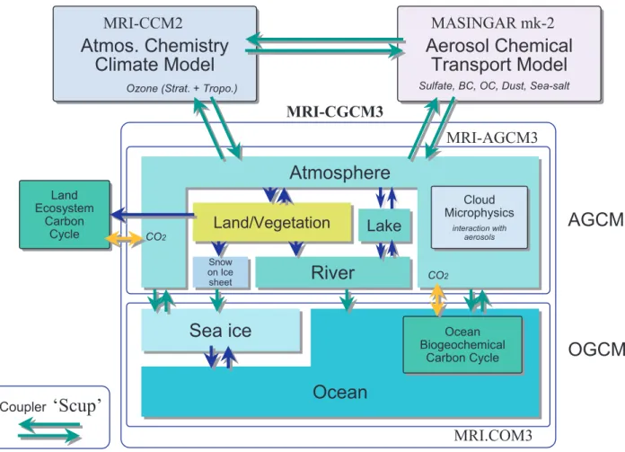
TheȱconfigurationȱofȱMRIȬESM1ȱisȱillustratedȱinȱFig.ȱ1.ȱTheȱatmosphere–oceanȱcoupledȱmodelȱ formingȱitsȱcoreȱcomponentȱisȱMRIȬCGCM3,ȱwhichȱitselfȱconsistsȱofȱMRI’sȱlatestȱAGCMȱandȱOGCMȱ versions.ȱTheȱAGCMȱincludesȱterrestrialȱbiosphereȱcarbonȱcycleȱprocesses,ȱandȱtheȱOGCMȱincludesȱ oceanȱbiogeochemicalȱprocesses.ȱTransportsȱandȱexchangesȱofȱatmosphericȱCO2ȱatȱtheȱlandȱandȱoceanȱ surfacesȱintegrateȱtheȱterrestrialȱandȱoceanȱcarbonȱcycles,ȱallowingȱrepresentationȱofȱtheȱglobalȱcarbonȱ cycle.ȱTheȱAGCMȱisȱcoupledȱwithȱanȱaerosolȱmodelȱandȱanȱatmosphericȱchemistry–climateȱmodelȱ (CCM)ȱ(focusedȱonȱozoneȱchemistry),ȱwhichȱallowsȱrepresentationȱofȱtheȱinteractionȱbetweenȱclimateȱ andȱvariationsȱinȱseveralȱaerosols,ȱozone,ȱandȱtraceȱgases.ȱNotȱonlyȱisȱtheȱCCMȱcoupledȱwithȱtheȱ AGCM,ȱtheȱaerosolȱmodelȱandȱtheȱCCMȱareȱcoupledȱwithȱeachȱother,ȱwhichȱenablesȱsimulationȱofȱ interactionsȱsuchȱasȱheterogeneousȱchemicalȱreactionsȱonȱaerosolȱsurfaces.ȱ

Figure 1 Configuration of the component models in MRI-ESM1. Green arrows denote data exchange with using Scup between the component models.

AGCM

OGCM

EcosystemLand Carbon

Cycle EcosystemLand

Carbon Cycle

Atmosphere Atmosphere Land/Vegetation

Land/Vegetation

on IceSnow sheet on IceSnow

sheet

River River

Lake Lake

Cloud Microphysics

interaction with aerosols

Cloud Microphysics

interaction with aerosols

CO2 CO2

Coupler

‘Scup’

MRI-CGCM3

MRI-AGCM3

Ocean Ocean Sea ice

Sea ice

Ocean

Biogeochemical Carbon Cycle

Ocean Biogeochemical

Carbon Cycle

MRI.COM3 Aerosol Chemical

Transport Model Aerosol Chemical

Transport Model

Sulfate, BC, OC, Dust, Sea-salt

MASINGAR mk-2 Atmos. Chemistry

Climate Model Atmos. Chemistry

Climate Model

Ozone (Strat. + Tropo.)

MRI-CCM2

TheȱAGCM,ȱcalledȱMRIȬAGCM3,ȱwasȱdevelopedȱatȱMRIȱ(Mizutaȱetȱal.,ȱ2006)ȱandȱisȱbasedȱonȱ JMA’sȱoperationalȱweatherȱpredictionȱmodel.ȱItsȱdynamicsȱframeworkȱusesȱaȱsemiȬLagrangianȱmethodȱ (Yoshimura,ȱinȱpreparation;ȱseeȱSectionȱ3.1)ȱthatȱhasȱtheȱimportantȱadvantagesȱofȱcomputationalȱ efficiencyȱandȱgoodȱconservationalȱpropertiesȱforȱmass,ȱstaticȱenergy,ȱandȱanyȱtracers.ȱInȱadditionȱtoȱtheȱ parameterizationsȱofȱtheȱoperationalȱmodel,ȱmanyȱnewȱorȱimprovedȱparameterizationsȱofȱvariousȱ physicalȱprocessesȱhaveȱbeenȱdeveloped.ȱInȱparticular,ȱnewȱparameterizationȱschemesȱforȱimportantȱ processes,ȱcumulusȱconvection,ȱradiation,ȱclouds,ȱtheȱplanetaryȱboundaryȱlayerȱ(PBL),ȱandȱterrestrialȱ hydrologyȱhaveȱbeenȱintroduced.ȱTheseȱnewlyȱintroducedȱschemesȱareȱincorporatedȱasȱoptionalȱ alternativesȱtoȱtheȱconventionalȱschemes.ȱ ȱ

Forȱcumulusȱconvection,ȱeitherȱaȱnewȱschemeȱdevelopedȱbyȱYoshimuraȱetȱal.ȱ(inȱpreparation;ȱseeȱ Sectionȱ3.2.2)ȱorȱaȱKainȬFritschȱschemeȱ(e.g.,ȱKainȱandȱFritsch,ȱ1990;ȱSectionȱ3.2.3)ȱcanȱbeȱselected,ȱorȱaȱ prognosticȱArakawaȬSchubertȬtypeȱ scheme,ȱwhichȱ wasȱmodifiedȱfromȱ theȱoriginalȱschemeȱ (e.g.,ȱ ArakawaȱandȱSchubert,ȱ1974;ȱRandallȱandȱPan,ȱ1993a,ȱ1993b)ȱforȱtheȱoperationalȱmodel.ȱForȱradiationȱ processes,ȱtheȱparameterizationȱschemeȱusedȱinȱtheȱoperationalȱmodelȱ(seeȱSectionȱ3.3)ȱhasȱbeenȱ introducedȱasȱanȱalternativeȱtoȱtheȱschemeȱusedȱinȱMRIȬCGCM2.3ȱ(ShibataȱandȱAoki,ȱ1989;ȱShibataȱandȱ Uchiyama,ȱ1992).ȱAȱcloudȱmicrophysicsȱschemeȱhasȱalsoȱbeenȱincorporatedȱintoȱMRIȬAGCM3ȱsoȱthatȱ theȱindirectȱeffectsȱofȱaerosolsȱonȱradiativeȱforcingȱcanȱbeȱrepresented.ȱThisȱcloudȱmicrophysicsȱschemeȱ isȱaȱtwoȬmomentȱbulkȱformulationȱ(Sectionȱ3.4)ȱthatȱexplicitlyȱrepresentsȱtwoȱconcentrations,ȱi.e.,ȱmassȱ (mixingȱratio)ȱandȱnumberȱconcentrations,ȱseparatelyȱforȱcloudȱdropletsȱandȱiceȱcrystals.ȱToȱmodelȱtheȱ PBL,ȱinȱadditionȱtoȱtheȱconventionalȱMellorȬYamadaȱ(MellorȱandȱYamada,ȱ1974)ȱlevelȱ2ȱscheme,ȱaȱ modificationȱofȱthatȱschemeȱdevelopedȱbyȱNakanishiȱ(2001)ȱandȱNakanishiȱandȱNiinoȱ(2004,ȱ2006,ȱ2009)ȱ (Sectionȱ3.5)ȱcanȱnowȱbeȱselected.ȱAȱnewȱlandȬsurfaceȱmodelȱcalledȱHALȱ(Hosaka,ȱinȱpreparation;ȱ Sectionȱ3.6)ȱhasȱbeenȱdevelopedȱthatȱcanȱhandleȱarbitraryȱnumbersȱofȱsnowȱandȱsoilȱlayersȱandȱmosaicȱ vegetationȱtypes,ȱandȱitȱallowsȱindividualȱpropertyȱparametersȱtoȱbeȱsetȱforȱspecialȱlandȬsurfaceȱtypesȱ suchȱasȱriceȱfieldsȱandȱurbanȱareas.ȱThisȱlandȬsurfaceȱmodelȱisȱmuchȱmoreȱflexibleȱthanȱthatȱinȱMRIȬ CGCM2.3,ȱwhichȱisȱaȱsimpleȱbiosphereȱmodelȱ(SiB:ȱSellersȱetȱal.,ȱ1986;ȱSatoȱetȱal.,ȱ1989)ȱmodifiedȱtoȱ handleȱmoreȱsoilȱlayersȱ(Hiraiȱetȱal.,ȱ2007).ȱRiverȱchannelsȱandȱlakesȱareȱalsoȱmodeledȱ(Sectionȱ3.8)ȱasȱ partȱofȱaȱclosedȱglobalȱwaterȱcycle.ȱ

TheȱoceanȱcomponentȱofȱMRIȬCGCM3ȱisȱaȱglobalȱversionȱofȱMRI.COM3ȱ(Tsujinoȱetȱal.,ȱ2010;ȱ Sectionȱ4)ȱdevelopedȱatȱMRIȱthatȱsupportsȱgeneralȱorthogonalȱcurvilinearȱcoordinates.ȱWeȱemployȱaȱ

tripolarȱcoordinateȱsystemȱthatȱdoesȱnotȱhaveȱtheȱNorthȱPoleȱasȱaȱsingularȱpoint,ȱbecauseȱMRIȬESM1ȱ coversȱtheȱworldȇsȱoceans,ȱincludingȱtheȱArcticȱOcean;ȱsouthȱofȱlatitudeȱ64°N,ȱtheȱcoordinateȱaxesȱ parallelȱlatitudeȱandȱlongitude.ȱAȱsophisticatedȱseaȬiceȱmodelȱwasȱintroducedȱinȱMRI.COM3,ȱfollowingȱ theȱ LosȱAlamosȱseaȬiceȱ modelȱ(CICE;ȱ HunkeȱandȱLipscomb,ȱ 2006),ȱwhichȱformulatesȱdynamicsȱ processesȱ suchȱ asȱ categorizedȱ thicknessȱ distribution,ȱ ridging,ȱ andȱ rheology,ȱ inȱ additionȱ toȱ theȱ thermodynamicsȱprocessesȱinȱtheȱseaȱiceȱmodelȱofȱMRIȬCGCM2.3,ȱwhichȱwasȱbasedȱonȱaȱfreeȬdriftȱ modelȱdevelopedȱbyȱMellorȱandȱKanthaȱ(1989).ȱ

Theȱaerosolȱmodel,ȱcalledȱMASINGARȱmkȬ2ȱ(Sectionȱ5),ȱisȱanȱadvancedȱversionȱofȱMASINGARȱ (Tanakaȱetȱal.,ȱ2003).ȱTheȱmodelȱhandlesȱfiveȱtypesȱofȱaerosols:ȱsulfate,ȱblackȱcarbon,ȱorganicȱcarbon,ȱ mineralȱdust,ȱandȱseaȱsalt.ȱForȱmineralȱdustȱandȱseaȱsalt,ȱtheȱaerosolsȱareȱcalculatedȱforȱseveralȱparticleȱ sizeȱbins.ȱProcessesȱrelatedȱtoȱaerosolsȱtreatedȱinȱtheȱmodelȱincludeȱnaturalȱandȱanthropogenicȱsources,ȱ chemicalȱreactionsȱinȱtheȱair,ȱtransport,ȱdiffusionȱandȱmixingȱbyȱatmosphericȱcirculationȱandȱconvection,ȱ andȱdryȱandȱwetȱdeposition.ȱ

TheȱatmosphericȱchemistryȱclimateȱmodelȱMRIȬCCM1ȱ(Shibataȱetȱal.,ȱ2005),ȱwhichȱwasȱdevelopedȱ atȱMRI,ȱprimarilyȱtargetsȱozoneȱinȱtheȱstratosphere.ȱTheȱversionȱincorporatedȱintoȱMRIȬESM1,ȱMRIȬ CCM2ȱ(DeushiȱandȱShibata,ȱ2010;ȱSectionȱ6),ȱisȱbasedȱonȱMRIȬCCM1,ȱbutȱtheȱnumberȱofȱchemicalȱ speciesȱandȱ(photo)ȱchemicalȱreactionsȱthatȱtheȱmodelȱcanȱhandleȱisȱexpanded,ȱallowingȱMRIȬCCM2ȱtoȱ simulateȱbothȱtroposphericȱandȱstratosphericȱozone.ȱMRIȬCCM2ȱcanȱbeȱcoupledȱwithȱtheȱMASINGARȱ mkȬ2ȱ aerosolȱmodel,ȱ whichȱenablesȱ theȱESMȱtoȱsimulateȱ chemical–aerosolȱ interactions,ȱ suchȱasȱ heterogeneousȱchemicalȱreactionsȱatȱtheȱaerosolȱsurface.ȱForȱexample,ȱtheȱeffectsȱofȱaȱstratosphericȱ aerosolȱderivedȱfromȱaȱvolcanicȱeruptionȱonȱstratosphericȱozoneȱbehaviorȱcanȱbeȱtakenȱintoȱaccount.ȱ

OneȱofȱtheȱmostȱimportantȱtargetsȱofȱESMsȱisȱtheȱglobalȱcarbonȱcycle,ȱwhichȱcomprisesȱmainlyȱ(atȱ leastȱonȱtimescalesȱofȱcenturiesȱupȱtoȱaȱmillennium)ȱterrestrialȱbiosphereȱcarbonȱcycleȱprocesses,ȱoceanȱ biogeochemicalȱ processes,ȱ surfaceȱ exchangeȱ andȱ transportȱ byȱ atmosphericȱ circulation,ȱ andȱ anthropogenicȱemissions.ȱTheȱchemicalȱcreationȱofȱCO²ȱinȱtheȱatmosphereȱ(calculatedȱbyȱMRIȬCCM2),ȱ thoughȱ itȱ isȱ aȱ veryȱ smallȱ amount,ȱ isȱ alsoȱ included.ȱ Twoȱ optionalȱ schemesȱ areȱ availableȱ forȱ parameterizationȱofȱterrestrialȱbiosphereȱcarbonȱcycleȱprocesses.ȱOneȱisȱaȱsimpleȱschemeȱthatȱusesȱ empiricalȱformulaeȱbasedȱonȱairȱandȱsoilȱtemperaturesȱandȱprecipitationȱ(Obata,ȱ2007).ȱTheȱotherȱisȱaȱ moreȱsophisticatedȱschemeȱthatȱtakesȱintoȱaccountȱphotosynthesisȱrelatedȱtoȱvegetationȱrepresentedȱbyȱ theȱlandȬsurfaceȱmodelȱ(Obata,ȱinȱpreparation;ȱSectionȱ8.1).ȱForȱoceanȱbiogeochemicalȱprocesses,ȱthereȱ

areȱalsoȱtwoȱoptions:ȱaȱsimpleȱmodelȱdevelopedȱbyȱObataȱandȱKitamuraȱ(2003),ȱandȱaȱmoreȱcomplexȱ schemeȱthatȱexplicitlyȱcalculatesȱnitrateȱ(i.e.,ȱnutrients),ȱphytoplankton,ȱzooplankton,ȱandȱdetritusȱ (Sectionȱ8.2).ȱTheȱintegratedȱlandȱandȱoceanȱcarbonȱcycleȱschemeȱintoȱMRIȬESM1ȱrealisticallyȱsimulatesȱ theȱexchangeȱofȱcarbonȱatȱtheȱlandȱorȱoceanȱsurfaceȱwithȱtheȱatmosphereȱ(CO²ȱflux)ȱandȱtheȱthreeȬ dimensionalȱ redistributionȱ ofȱ theȱ alteredȱ atmosphericȱ CO2ȱ concentrationȱ byȱ processesȱ suchȱ asȱ advection,ȱverticalȱmixingȱdueȱtoȱdiffusion,ȱandȱcumulusȱconvection.ȱ

AnȱESMȱgenerallyȱconsistsȱofȱaȱnumberȱofȱcomplexȱcomponents,ȱeachȱofȱwhichȱisȱindependentlyȱ developedȱbyȱaȱspecializedȱmodelingȱgroup,ȱandȱtheȱcomponentȱmodelsȱmustȱworkȱtogether.ȱForȱ efficientȱdevelopment,ȱitȱmustȱbeȱpossibleȱtoȱintegrateȱtheȱcomponentȱmodelsȱintoȱtheȱESMȱwithoutȱanyȱ troublesomeȱmodificationȱbeingȱrequired.ȱOneȱofȱtheȱmostȱimportantȱstrongȱpointsȱofȱMRIȬESM1ȱisȱthatȱ theȱcomponentȱmodelsȱcanȱbeȱflexiblyȱcoupledȱwithȱtheȱScupȱcouplerȱ(YoshimuraȱandȱYukimoto,ȱ2008;ȱ Sectionȱ9).ȱScupȱallowsȱtheȱflexibleȱexchangeȱofȱdataȱbetweenȱcomponentȱmodelsȱwithȱdifferentȱ resolutionsȱorȱgridȱcoordinatesȱandȱdifferentȱtimeȱintervals.ȱTheȱdataȱexchange,ȱmoreover,ȱisȱdoneȱwithȱ goodȱconservationȱofȱbothȱthreeȬdimensionalȱdataȱandȱhorizontalȱtwoȬdimentionalȱdata,ȱwhichȱisȱ essentialȱforȱclimateȱmodelsȱandȱESMs.ȱThisȱfunctionalityȱmeansȱthatȱMRIȬESM1ȱcanȱperformȱtheȱmanyȱ kindsȱofȱexperimentsȱplannedȱforȱCMIP5ȱbyȱflexibleȱconfigurationȱofȱtheȱcomponentȱmodelsȱandȱ parameterizationȱschemes.ȱ

3. Atmospheric model (MRI-AGCM3)

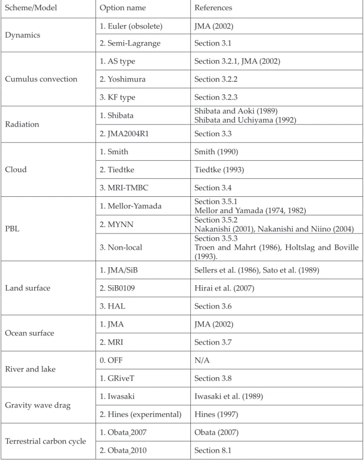
Theȱatmosphericȱcomponentȱ(includingȱlandȱandȱoceanȱsurfaces)ȱmodel,ȱMRIȬAGCM3,ȱwasȱ developedȱ fromȱ aȱ modelȱ byȱ Mizutaȱ etȱ al.ȱ (2006)ȱ byȱ theȱ additionȱ ofȱ aȱ numberȱ ofȱ physicalȱ parameterizationȱoptionsȱandȱimprovements,ȱsummarizedȱinȱTableȱ1.ȱTheȱdynamicsȱframeworkȱofȱ MRIȬAGCM3,ȱwhichȱMizutaȱetȱal.ȱ(2006)ȱdidȱnotȱdocumentȱinȱdetail,ȱisȱdescribedȱinȱSectionȱ3.1.ȱInȱtheȱ subsequentȱsections,ȱtheȱmajorȱphysicalȱparameterizationsȱdevelopedȱforȱMRIȬAGCM3ȱareȱdescribed:ȱ cumulusȱconvectionȱ(Sectionȱ3.2),ȱradiationȱ(Sectionȱ3.3),ȱcloudȱmodelȱ(Sectionȱ3.4),ȱPBLȱ(Sectionȱ3.5),ȱ landȬsurfaceȱmodelȱ(Sectionȱ3.6),ȱoceanȱsurfaceȱprocessesȱ(Sectionȱ3.7),ȱandȱriver–lakeȱmodelȱ(Sectionȱ 3.8).ȱOtherȱcomponentsȱofȱMRIȬAGCM3ȱareȱbasicallyȱtheȱsameȱasȱinȱtheȱoriginalȱmodelȱofȱMizutaȱetȱal.ȱ (2006).ȱ

ȱ

3.1. Dynamics framework

InȱtheȱMRIȬAGCM3ȱglobalȱspectralȱatmosphericȱmodel,ȱhydrostaticȱprimitiveȱequationsȱareȱusedȱ asȱprognosticȱequations.ȱAȱtwoȬtimeȬlevelȱsemiȬimplicitȱsemiȬLagrangianȱschemeȱisȱusedȱforȱtimeȱ integration.ȱThisȱschemeȱpermitsȱaȱlongerȱtimeȬstepȱthanȱtheȱformerlyȱusedȱsemiȬimplicitȱEulerianȱ schemeȱandȱrealizesȱhighȱefficiency.ȱTheȱverticallyȱconservativeȱsemiȬLagrangianȱadvectionȱschemeȱisȱ alsoȱgloballyȱconservativeȱandȱthereforeȱsuitableȱnotȱonlyȱforȱshortȬtermȱweatherȱpredictionsȱbutȱalsoȱ forȱlongȬtimeȬperiodȱintegrationsȱsuchȱasȱexperimentsȱforȱprojectingȱclimateȱchange.ȱ

TheȱprognosticȱequationsȱareȱgivenȱinȱSectionȱ3.1.1,ȱtheȱverticallyȱconservativeȱsemiȬLagrangianȱ schemeȱisȱexplainedȱinȱSectionȱ3.1.2,ȱandȱtheȱtimeȱintegrationȱschemeȱisȱdescribedȱinȱSectionȱ3.1.3.ȱ

3.1.1. Prognostic equations

Theȱfollowingȱhydrostaticȱprimitiveȱequationsȱareȱusedȱasȱprognosticȱequations.ȱ

¸¸ 0

¹

¨¨ ·

© §

¸¸¹

¨¨ ·

©

˜§

’

¸¸

¹

¨¨ ·

©

§

wK Kw wK

w wK w wK

w w

w p p p

t v^H (3.1)

q

H q q P

tq dt

dq{ ˜’

wK K w w

w v

(3.2)ȱ

dT

dt F_T P_T K_T

(3.3)ȱ

Table 1. List of MRI-AGCM3 options

Scheme/Modelȱ Optionȱnameȱ Referencesȱ

1.ȱEulerȱ(obsolete)ȱ JMAȱ(2002)ȱ ȱ Dynamicsȱ

2.ȱSemiȬLagrangeȱ Sectionȱ3.1ȱ

1.ȱASȱtypeȱ Sectionȱ3.2.1,ȱJMAȱ(2002)ȱ 2.ȱYoshimuraȱ Sectionȱ3.2.2ȱ

Cumulusȱconvectionȱ

3.ȱKFȱtypeȱ Sectionȱ3.2.3ȱ

1.ȱShibataȱ ShibataȱandȱAokiȱ(1989)ȱ ShibataȱandȱUchiyamaȱ(1992)ȱ Radiationȱ

2.ȱJMA2004R1ȱ Sectionȱ3.3ȱ

1.ȱSmithȱ Smithȱ(1990)ȱ

2.ȱTiedtkeȱ Tiedtkeȱ(1993)ȱ Cloudȱ

3.ȱMRIȬTMBCȱ Sectionȱ3.4ȱ 1.ȱMellorȬYamadaȱ Sectionȱ3.5.1ȱ

MellorȱandȱYamadaȱ(1974,ȱ1982)ȱ

2.ȱMYNNȱ Sectionȱ3.5.2ȱ

Nakanishiȱ(2001),ȱNakanishiȱandȱNiinoȱ(2004)ȱ PBLȱ

3.ȱNonȬlocalȱ

Sectionȱ3.5.3ȱ

TroenȱandȱMahrtȱ(1986),ȱHoltslagȱandȱBovilleȱ (1993).ȱ

1.ȱJMA/SiBȱ Sellersȱetȱal.ȱ(1986),ȱSatoȱetȱal.ȱ(1989)ȱ 2.ȱSiB0109ȱ ȱ Hiraiȱetȱal.ȱ(2007)ȱ

Landȱsurfaceȱ

3.ȱHALȱ Sectionȱ3.6ȱ

1.ȱJMAȱ JMAȱ(2002)ȱ ȱ

Oceanȱsurfaceȱ

2.ȱMRIȱ Sectionȱ3.7ȱ

0.ȱOFFȱ N/Aȱ

Riverȱandȱlakeȱ

1.ȱGRiveTȱ Sectionȱ3.8ȱ

1.ȱIwasakiȱ Iwasakiȱetȱal.ȱ(1989)ȱ Gravityȱwaveȱdragȱ

2.ȱHinesȱ(experimental)ȱ Hinesȱ(1997)ȱ 1.ȱObataȱ2007ȱ Obataȱ(2007)ȱ Terrestrialȱcarbonȱcycleȱ

2.ȱObataȱ2010ȱ Sectionȱ8.1ȱ

>

^{c Tc q}

@

^p

F

pd pv

T { 1 N vZ1

(3.3a)ȱ

ȱ ȱ

d v

_H

2: u r

dt F

_vH

P

_vH

K

_vHȱ ȱ ȱ (3.4)ȱ

ȱ ȱ ȱ ȱ ȱ ȱ

F

_vH

{ ’) R

_d

T

_v

’ ln p

ȱ ȱ ȱ (3.4a)ȱ

ȱ ȱ wK

w wK

w p

p T R_{d v} )

ȱ ȱ ȱ (3.5)ȱ

ȱ ȱ T_v {T 1 R_v

R_d 1

§

©¨ ·

¹¸q

­®

¯

½¾

¿^{.ȱ ȱ ȱ (3.6)ȱ}

Here,ȱtheȱfollowingȱnotationsȱareȱused.ȱ

t

_{ȱ :ȱTimeȱ} pȱ :ȱPressureȱ

p_sȱ :ȱSurfaceȱpressureȱ

K

ȱ :ȱHybridȱ p

V

ȱverticalȱcoordinateȱ(

V

{ p p_s)ȱ

K

ȱ :ȱ

K

{d

K

dtȱ v_Hȱ :ȱHorizontalȱwindȱ

qȱ :ȱWaterȱvaporȱmixingȱratioȱ

T

ȱ :ȱTemperatureȱ T_vȱ :ȱVirtualȱtemperatureȱ R_dȱ :ȱGasȱconstantȱofȱdryȱairȱ R_vȱ :ȱGasȱconstantȱofȱwaterȱvaporȱ

c

_pdȱ :ȱSpecificȱheatȱofȱdryȱairȱatȱconstantȱpressureȱ

c

_pvȱ :ȱSpecificȱheatȱofȱwaterȱvaporȱatȱconstantȱpressureȱ

Z

ȱ :ȱVerticalȱpressureȱatȱ pȱcoordinate,ȱ

Z

{dp dtȱ

N

ȱ :ȱ

N { R

_d

c

_pdȱ

F_Tȱ :ȱHeatingȱbyȱadiabaticȱcompressionȱ(expansion)ȱ

F

_vHȱ :ȱPressureȱgradientȱforceȱ

P

_q,P_T,

P

_v

H:ȱContributionȱbyȱphysicalȱprocessesȱ K_T,

K

_vHȱ :ȱHorizontalȱviscosityȱ

:

ȱ :ȱAngularȱvelocityȱofȱtheȱrotationȱofȱtheȱearthȱ

rȱ :ȱPositionȱvectorȱfromȱtheȱcenterȱofȱtheȱearthȱ

’

ȱ :ȱHorizontalȱgradientȱonȱtheȱ

K

ȱsurface.ȱ

Theȱ

K

ȱcoordinateȱisȱaȱhybridȱverticalȱcoordinateȱthatȱsteadilyȱchangesȱfromȱtheȱterrainȱfollowingȱ

V

ȱcoordinateȱnearȱtheȱsurfaceȱtoȱtheȱ pȱcoordinateȱnearȱtheȱtopȱ(SimmonsȱandȱBurridge,ȱ1981).ȱ

K K p, p

_s

^{ȱisȱaȱmonotonicȱfunctionȱofȱ pȱthatȱsatisfiesȱ}

^{K 0, p}

s

⁰

^ȱandȱ

^{K p}

s

, p

_s

¹

^{.ȱ pȱcanȱbeȱ}

definedȱasȱaȱfunctionȱofȱ

K

ȱandȱ p_s,ȱandȱ

A K

ȱandȱ

B K

ȱareȱintroducedȱtoȱsatisfyȱ

p K , p

_s

^{A K B K ˜ p}

s.ȱ (3.7)ȱ

A K 0

ȱisȱsatisfiedȱinȱtheȱlowerȱlayersȱnearȱtheȱsurfaceȱ(

V

Ȭcoordinate),ȱandȱ

B K 0

ȱisȱsatisfiedȱinȱ theȱupperȱlayersȱ(pȬcoordinate).ȱ

3.1.2. Advection with a vertically conservative semi-Lagrangian scheme

Theȱ verticallyȱ conservativeȱ semiȬLagrangianȱ schemeȱ (brieflyȱ describedȱ byȱ Yoshimuraȱ andȱ Matsumura,ȱ2003,ȱ2005)ȱisȱusedȱforȱtheȱadvectionȱcalculation.ȱTheȱequationȱ

0

’

˜

q q

tq ^H wK

K w w

w v (3.8)

isȱusedȱtoȱexplainȱtheȱcalculationȱofȱtheȱadvectionȱofȱ q.ȱEquationȱ(3.8)ȱisȱtheȱsameȱasȱEq.ȱ(3.2)ȱexceptȱ thatȱtheȱrightȬhandȱsideȱofȱEq.ȱ(3.8)ȱisȱ0ȱtoȱsimplifyȱitsȱexplanation.ȱTheȱadvectionȱofȱ

T

ȱandȱ v_H,ȱEqs.ȱ (3.3)ȱandȱ(3.4),ȱisȱcalculatedȱinȱbasicallyȱtheȱsameȱwayȱasȱthatȱofȱ q.ȱFromȱEqs.ȱ(3.1)ȱandȱ(3.8),ȱ

¸¸ 0

¹

¨¨ ·

© §

¸¸¹

¨¨ ·

©

˜§

’

¸¸

¹

¨¨ ·

©

§ pq

pq pq

t ^H wK

Kw wK

w wK w wK

w w

w v (3.9)

isȱderived,ȱwhichȱisȱtheȱconservationȱequationȱofȱwaterȱvapor.ȱWhenȱ

q 1

,ȱEq.ȱ(3.9)ȱisȱtheȱsameȱasȱEq.ȱ (3.1),ȱtheȱmassȱconservationȱequation.ȱFromȱEqs.ȱ(3.1)ȱandȱ(3.9),ȱ

¸¸¹

¨¨ ·

© §

¸¸

¹

¨¨ ·

©

§

wK Kw wK

w wK w wK

w p p

p D dt d_H

(3.10)

¸¸¹

¨¨ ·

© §

¸¸

¹

¨¨ ·

©

§ pq

pq D pq

dt d_H

wK Kw wK

w wK w wK

w (3.11)

areȱderived,ȱwhereȱ d_H dt{w wtv_H˜’ȱrepresentsȱhorizontalȱadvectionȱandȱ D{ ’ ˜v_Hȱrepresentsȱ horizontalȱdivergence.ȱ

Equationsȱ(3.10)ȱandȱ(3.11)ȱareȱverticallyȱdiscretized.ȱThereȱareȱKȱfullȱlevelsȱinȱtheȱverticalȱdirectionȱ

andȱ v_H,T,qȱareȱpositionedȱatȱeachȱfullȱlevelȱ(k 1, 2, 3, ...,K).ȱ

K

ȱisȱpositionedȱatȱtheȱhalfȱlevelsȱ (k 1 2, 3 2, 5 2, ...,K1 2),ȱwhichȱareȱtheȱboundariesȱbetweenȱtheȱfullȱlevels.ȱAtȱtheȱlowerȱboundaryȱ (k 1 2),ȱ p p_s,ȱ

K 1

,ȱandȱ

K 0

ȱareȱsatisfied.ȱAtȱtheȱupperȱboundaryȱ(k K1 2),ȱ

p 0

,ȱ

K 0

,ȱ andȱ

K 0

ȱareȱsatisfied.ȱFromȱEq.ȱ(3.7),ȱtheȱpressureȱatȱtheȱhalfȱlevelȱisȱobtainedȱbyȱ

p

_{k1 2}

A

_{k1 2}

B

_{k1 2}

p

_s

.

(3.12)ȱ

Equationsȱ(10)ȱandȱ(11)ȱareȱverticallyȱdiscretizedȱ(integratedȱfromȱ k1 2ȱtoȱ k1 2)ȱasȱ

2 1 2

1

¸¸¹

¨¨ ·

© §

¸¸¹

¨¨ ·

© § ' '

k k

k k

H k p p

p D dt p

d

wK Kw wK

Kw (3.13)ȱ

2 1 2

1

¸¸¹

¨¨ ·

© §

¸¸¹

¨¨ ·

© § ' '

k k

k k k k

H k pq

pq q

p D q dt p d

wK Kw wK

Kw ,ȱ ȱ (3.14)ȱ

whereȱ 'p_kȱisȱdefinedȱasȱ

'p

_k

{ p

_{k1 2}

p

_{k1 2}.ȱ (3.15)ȱ

TheȱleftȬhandȱsidesȱofȱEqs.ȱ(3.13)ȱandȱ(3.14)ȱrepresentȱhorizontalȱadvection,ȱtheȱfirstȱtermsȱonȱtheȱrightȬ handȱsidesȱrepresentȱhorizontalȱdivergenceȱ(convergence),ȱandȱtheȱsecondȱandȱthirdȱtermsȱonȱtheȱrightȬ handȱsidesȱrepresentȱverticalȱflux.ȱ

ThreeȬdimensionalȱadvectionȱisȱcalculatedȱbyȱexecutingȱtheȱtimeȱintegrationȱofȱtheseȱequationsȱinȱ theȱfollowingȱorder:ȱ

Ԙ Horizontalȱdivergence ԙ Vertical flux

Ԛ Horizontalȱadvection ԛ Verticalȱflux

Ԝ Horizontalȱdivergence.

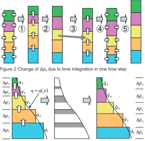
Figureȱ2ȱshowsȱtheȱchangeȱinȱ 'p_kȱdueȱtoȱtheȱtimeȱintegrationȱofȱEq.ȱ(3.13).ȱTheȱverticalȱfluxȱ(stepsȱԙ and ԛ) isȱcalculatedȱbyȱtheȱconservativeȱsemiȬLagrangianȱscheme.ȱFigureȱ3ȱshowsȱchangesȱinȱ 'p_kȱ andȱ q_kȱdueȱtoȱtheȱverticalȱflux.ȱTheȱdiagramȱonȱtheȱleftȱshowsȱ 'p_kȱandȱ q_kȱbeforeȱtheȱverticalȱfluxȱ calculation.ȱTheȱdistributionȱofȱ

q q p

ȱisȱobtainedȱfromȱ q_k,ȱwhichȱsatisfiesȱ

q p dp

p_{k1/ 2} p_{k1/ 2}

³ ^q

k

'p

_k.ȱ (3.16)ȱ

TheȱhatchedȱpartȱofȱtheȱdiagramȱinȱtheȱcenterȱofȱFig.ȱ3ȱrepresentsȱ qȱmovingȱtoȱtheȱupperȱlayer.ȱTheȱ valuesȱofȱ '˜p_kȱandȱ q˜_kȱafterȱtheȱverticalȱfluxȱcalculationȱareȱshownȱinȱtheȱrightȱdiagram.ȱ q˜_kȱisȱ calculatedȱasȱ

˜ q_k 1

'˜p_k q p dp

˜ p_{k1/ 2}

˜ p_{k1/ 2}

³ ^.

^(3.17)ȱ

Inȱtheȱactualȱcalculation,ȱtheȱintegratedȱvalueȱfromȱtheȱupperȱboundaryȱ Q p q p dp

0

³

p ^{ȱ (3.18)ȱ}

isȱusedȱinsteadȱofȱ

q p

ȱtoȱmakeȱtheȱcalculationȱfaster.ȱTheȱvaluesȱofȱ

Q

ȱatȱtheȱhalfȱlevelsȱareȱobtainedȱ fromȱ

³

¦

^{K '}

k l

l l pk

k q pdp q p

p Q

1 2

/ 1 2 0

/

1 ȱ (3.19)ȱ

Thereȱareȱ severalȱmethodsȱforȱcalculatingȱtheȱdistributionȱofȱ

Q p

ȱfromȱ

Q p

_{k1/ 2}

^{ȱandȱ q}k.ȱToȱ calculateȱmaterialȱtransport,ȱsuchȱasȱofȱwaterȱvapor,ȱtheȱPiecewiseȱRationalȱMethodȱ(PRM;ȱXiaoȱandȱ Peng,ȱ2004),ȱaȱmonotonicȱandȱconservativeȱmethod,ȱisȱused.ȱForȱtheȱadvectionȱofȱ

T

ȱandȱ v_H,ȱtheȱcubicȱ Lagrangeȱinterpolationȱmethodȱisȱused.ȱ

Q p ˜

_{k1/ 2}

^ȱisȱobtainedȱfromȱtheȱ

Q p

ȱdistribution,ȱandȱ q˜_kȱisȱ calculatedȱfromȱ

˜ q_k 1

'˜p_k

^

Q

p˜_{k1/ 2}

^Q

^p˜k1/ 2

` ^,

^(3.20)ȱ

whichȱisȱderivedȱfromȱEqs.ȱ(3.17)ȱandȱ(3.18).ȱ

Figure 2 Change of ǻpk due to time integration in one time step

Figure 3 Change of ǻpk and q before and after vertical flux calculation

Thisȱschemeȱforȱtheȱverticalȱfluxȱcalculationȱisȱbasicallyȱtheȱsameȱasȱthatȱforȱtheȱverticalȱcoordinateȱ transformationȱinȱtheȱScupȱcouplerȱ(YoshimuraȱandȱYukimoto,ȱ2008).ȱTheȱverticalȱfluxȱcalculationȱcanȱ alsoȱbeȱconsideredȱaȱverticalȱcoordinateȱtransformation.ȱ

Inȱstep Ԛ, theȱhorizontalȱadvection isȱcalculatedȱbyȱaȱconventionalȱsemiȬLagrangianȱscheme.ȱAȱ quasiȬcubicȱinterpolationȱmethodȱ(Ritchieȱetȱal.,ȱ1995)ȱisȱusedȱforȱhorizontalȱinterpolation.ȱAȱquasiȬfifthȬ orderȱinterpolationȱmethodȱisȱusedȱonlyȱforȱtheȱadvectionȱofȱhorizontalȱwind,ȱtoȱimproveȱprecision.ȱAȱ correctionȱmethodȱsimilarȱtoȱthatȱdescribedȱbyȱPriestleyȱ(1993)ȱandȱbyȱGravelȱandȱStaniforthȱ(1994)ȱisȱ usedȱforȱglobalȱconservationȱinȱtheȱcalculationȱofȱmaterialȱadvection.ȱ

ȱ

3.1.3. Time integration method

AȱgeneralizedȱprognosticȱequationȱfromȱEqs.ȱ(3.1)ȱthroughȱ(3.4),ȱ dX

dt F X

,

(3.21)ȱ

isȱconsidered.ȱAȱtwoȬtimeȬlevelȱsemiȬimplicitȱsemiȬLagrangianȱschemeȱ(e.g.,ȱTempertonȱetȱal.,ȱ2001)ȱandȱ SETTLSȱ(Hortal,ȱ2002)ȱareȱadoptedȱtoȱdiscretizeȱEq.ȱ(3.21)ȱasȱ

X

X

_D⁰

't

1

2 ^ F

⁽⁾

E L

⁰

L

`

_D

¹ ₂ ^ ^F

⁰

^{E L}

⁰

^L

`

^{ȱ (3.22)ȱ ȱ}

F

⁽⁾

{ 2F

⁰

F

,ȱ (3.23)ȱ

whereȱ

't

ȱisȱaȱtimeȬstep;ȱ

L X

ȱisȱtheȱlinearizedȱtermȱofȱ

F X

;ȱtheȱsubscriptȱDȱmeansȱtheȱthreeȬ dimensionalȱdepartureȱpoint;ȱtheȱsuperscriptsȱ–,ȱ0,ȱandȱ+ȱmeanȱpastȱtimeȱ

(t 't)

,ȱpresentȱtimeȱ

(t)

,ȱ andȱ futureȱ timeȱ

(t 't)

,ȱrespectively;ȱ andȱ theȱsuperscriptȱ(+)ȱmeansȱtheȱ futureȱ timeȱbyȱtimeȱ extrapolation.ȱ

E

ȱisȱaȱsecondȬorderȱdecenteringȱparameterȱandȱisȱsetȱtoȱ1.2,ȱslightlyȱlargerȱthanȱ1.0,ȱ whichȱenhancesȱtheȱstabilizingȱeffectȱofȱtheȱsemiȬimplicitȱscheme.ȱSinceȱtheȱrightȬhandȱsideȱofȱEq.ȱ(3.22)ȱ isȱtheȱtimeȱaverageȱofȱtheȱpresentȱtimeȱandȱtheȱfutureȱtimeȱandȱtheȱspatialȱaverageȱofȱtheȱdepartureȱ pointȱandȱtheȱarrivalȱpoint,ȱEq.ȱ(3.22)ȱhasȱsecondȬorderȱprecisionȱinȱtimeȱandȱspace.ȱEquationȱ(3.22)ȱisȱ transformedȱasȱ

X1

2

E

'tL X⁰1

2't F

^

⁽⁾

E

L⁰L

`

ª

¬« º

¼»

D

1

2't F

^

⁰

E

L⁰

`

^{.ȱ (3.24)ȱ}

TheȱrightȬhandȱsideȱofȱEq.ȱ(3.24)ȱisȱcalculatedȱexplicitly.ȱTheȱvalueȱatȱtheȱthreeȬdimensionalȱdepartureȱ

pointȱisȱobtainedȱbyȱtheȱadvectionȱcalculationȱwithȱtheȱverticallyȱconservativeȱsemiȬLagrangianȱscheme.ȱ Sinceȱ

L

ȱisȱaȱlinearȱfunctionȱofȱ

X

,ȱ

X

ȱcanȱbeȱobtainedȱfromȱEq.ȱ(3.24).ȱInȱspectralȱmodels,ȱEq.ȱ(3.24)ȱ canȱbeȱsolvedȱindependentlyȱofȱtheȱhorizontalȱwavenumberȱandȱthereforeȱ

X

ȱcanȱbeȱobtainedȱeasily.ȱ

3.2. Cumulus convection

3.2.1. Arakawa-Schubert-type scheme

TheȱArakawaȬSchubertȱ(AS)Ȭtypeȱschemeȱ(ArakawaȱandȱSchubert,ȱ1974),ȱoneȱofȱtheȱmostȱpopularȱ forȱcumulusȱconvectionȱparameterization,ȱisȱbasedȱonȱtheȱassumptionȱthatȱthereȱexistsȱanȱensembleȱ(orȱ group)ȱofȱcumulusȱcloudsȱatȱvariousȱheightsȱinȱoneȱgridȱcolumnȱofȱtheȱmodel,ȱandȱthatȱeachȱindividualȱ cumulusȱcloudȱofȱtheȱensembleȱoccupiesȱaȱsufficientlyȱsmallȱareaȱofȱtheȱgrid.ȱTheȱupdraftȱwithinȱtheȱ cumulusȱconvection,ȱbyȱwhichȱheatȱandȱmoistureȱareȱcarriedȱtoȱtheȱupperȱlevelȱwhileȱcondensingȱtheȱ saturatedȱmoisture,ȱandȱdryȱcoldȱairȱfromȱtheȱsurroundingsȱisȱtakenȱinȱ(aȱprocessȱcalledȱentrainment),ȱ isȱparameterizedȱbyȱtheȱcloudȱmodel.ȱTheȱgenerationȱofȱconvectionȱandȱitsȱstrengthȱareȱdeterminedȱbyȱ theȱdestabilizationȱofȱtheȱgridȬscaleȱstratification,ȱwhichȱisȱevaluatedȱbyȱtheȱcloudȱworkȱfunctionȱ (ArakawaȱandȱSchubert,ȱ1974).ȱTheȱensembleȱeffectȱofȱtheȱcumulusȱconvectionȱonȱtheȱcompensatedȱ subsidenceȱandȱcloudȱtopȱdetrainmentȱisȱparameterizedȱbyȱtheȱcloudȱmassȱfluxȱmethod.ȱTheȱJMA’sȱ operationalȱscheme,ȱthoughȱbasedȱonȱtheȱoriginalȱschemeȱofȱArakawaȱandȱSchubertȱ(1974),ȱhasȱbeenȱ improvedȱandȱdevelopedȱvariously.ȱ

Someȱofȱtheȱmodificationsȱareȱtheȱfollowing:ȱ

1.  AȱprognosticȱmassȱfluxȱmethodȱisȱusedȱtoȱexpressȱtheȱconditionȱofȱawayȱfromȱquasiȬ equilibriumȱ(RandallȱandȱPan,ȱ1993a,ȱ1993b;ȱPanȱandȱRandall,ȱ1993,ȱ1998)ȱ ȱ

2.  Theȱcumulusȱdowndraftȱisȱalsoȱconsideredȱ(ChengȱandȱArakawa,ȱ1997).ȱ

3.ȱ Aȱ midȬlevelȱ convectionȱ schemeȱ isȱ includedȱ toȱ expressȱ theȱ midȬlatitudeȱ convectionȱ accompanyingȱtheȱfrontȱandȱsynopticȬscaleȱdisturbances.ȱ

Cumulus updraft

InȱanȱASȬtypeȱscheme,ȱanȱensembleȱofȱcumulusȱcloudsȱatȱvariousȱheightsȱisȱassumed,ȱwhichȱtheȱ cloudȱbaseȱisȱatȱtheȱtopȱofȱtheȱboundaryȱlayer.ȱTheȱprognosticȱequationsȱforȱtheȱcloudȱbaseȱmassȱfluxȱ areȱasȱfollows:ȱ

³

³

Z^Z_B^T

p T u

Z ZB

u

T dz C

s gs T dz

T gT

A K K

ȱ

(3.25)ȱ

) , (

_B^u

u

B

F A M

t M w

w ȱ

(3.26)

ȱ

HereȱAȱisȱtheȱcloudȱworkȱfunction;ȱT^uȱandȱs^uȱareȱtheȱtemperatureȱandȱtheȱdryȱstaticȱenergy,ȱ respectively,ȱofȱaȱparcelȱinȱtheȱcumulusȱupdraft;ȱTȱandȱsȱareȱtheȱtemperatureȱandȱdryȱstaticȱenergy,ȱ respectively,ȱofȱtheȱenvironment;ȱM^uBȱisȱtheȱcloudȱbaseȱmassȱflux;ȱandȱ΋ȱisȱtheȱstandardizedȱmassȱflux,ȱ whichȱdependsȱonȱtheȱcloudȱbaseȱmassȱflux.ȱFȱisȱtheȱfunctionȱofȱtheȱdampingȱformulationȱbasedȱonȱ RandallȱandȱPanȱ(1993a,ȱ1993b)ȱandȱPanȱandȱRandallȱ(1998).ȱSomeȱmodificationsȱofȱfunctionȱFȱareȱ adoptedȱinȱMRIȬAGCM3.ȱTheȱtopȱofȱeachȱcumulusȱcloudȱcorrespondsȱtoȱoneȱverticalȱlevelȱinȱtheȱmodel,ȱ andȱtheȱensembleȱsizeȱ(i.e.,ȱtheȱnumberȱofȱcumulusȱclouds)ȱdependsȱonȱtheȱverticalȱresolutionȱofȱtheȱ model.ȱ

Inȱeachȱcumulusȱcloud,ȱanȱentrainmentȱrateȱΏȱandȱaȱmassȱfluxȱM^uȱisȱassumed:ȱ

dz O dM M

u u

1

(3.27)

so,ȱ

)) (

exp(

_B

u B

u

M z z

M O

(3.28)

TheȱsuffixȱBȱrefersȱtoȱtheȱcloudȱbaseȱlevel.ȱ

Toȱreduceȱcomputationalȱcosts,ȱEq.ȱ(3.28)ȱisȱlinearizedȱfollowingȱMoorthiȱandȱSuarezȱ(1992),ȱ

K

O

_{B B}^u

u B

u

M z z M

M ( 1 ( )) .

(3.29)

ȱ

Therefore,ȱtheȱsubȬgridȬscaleȱvaluesȱofȱeachȱcumulusȱcloud,ȱsuchȱasȱtheȱmassȱfluxȱandȱentrainmentȱrateȱ andȱtheȱcloudȱworkȱfunction,ȱcanȱbeȱestimatedȱfromȱtheȱgridȬscaleȱvaluesȱofȱtheseȱparameters.ȱTheȱ cloudȱbaseȱmassȱfluxȱMBȱisȱaȱroleȱofȱtheȱclosureȱinȱtheȱASȱparameterization.ȱInȱMRIȬAGCM3,ȱtheȱcloudȱ baseȱisȱfixedȱandȱitȱisȱassumedȱthatȱdetrainmentȱoccursȱonlyȱfromȱtheȱcloudȱtop.ȱAdditionally,ȱaȱ minimumȱvalueȱofȱ

Ώ

ȱisȱset,ȱandȱaȱcumulusȱcloudȱwithȱ

Ώ

ȱ=ȱ0ȱisȱexcludedȱ(Tokiokaȱetȱal.,ȱ1988).ȱ ȱ

ȱ ȱ

Cumulus downdraft

Inȱconvectiveȱclouds,ȱthereȱareȱnotȱonlyȱaȱverticalȱupdraftȱbutȱalsoȱaȱstrongȱdowndraft,ȱcausedȱbyȱ coolingȱdueȱtoȱevaporationȱofȱraindropsȱandȱtheȱloadingȱofȱprecipitationȱparticles.ȱHeatingȱandȱdryingȱ ofȱtheȱlowerȱlayerȱbecomeȱexcessive,ȱcomparedȱwithȱobservation,ȱifȱthisȱdowndraftȱisȱnotȱconsideredȱ (ArakawaȱandȱCheng,ȱ1993),ȱsoȱitȱisȱnecessaryȱtoȱparameterizeȱit.ȱInȱMRIȬAGCM3,ȱaȱsimplifiedȱmethodȱ insteadȱofȱthatȱofȱArakawaȱandȱChengȱ(1993)ȱisȱused.ȱTheȱcumulusȱdowndraftȱisȱexpressedȱnotȱasȱaȱ cloudȱensembleȱlikeȱtheȱcumulusȱupdraftȱbutȱasȱaȱsingleȱcumulusȱcloud.ȱTheȱdowndraftȱisȱassumedȱtoȱ startȱfromȱaȱheightȱthatȱisȱaboveȱtheȱcloudȱbaseȱandȱwhereȱtheȱcloudȱbaseȱmassȱfluxȱofȱtheȱupdraftȱ becomesȱhalfȱ.ȱ

Itȱisȱalsoȱassumedȱthatȱentrainmentȱandȱdetrainmentȱratesȱhaveȱtheȱsameȱvaluesȱaboveȱtheȱcloudȱ baseȱandȱonlyȱtheȱdetrainmentȱrateȱisȱconsideredȱbeneathȱtheȱcloudȱbase.ȱ

Mid-level convection

ConvectionȱdueȱtoȱfrontalȱsystemȱandȱmidȬlatitudeȱsynopticȬscaleȱdisturbancesȱisȱnotȱexpressibleȱ withȱanȱASȬtypeȱschemeȱbecauseȱthatȱschemeȱassumesȱthatȱtheȱcloudȱbaseȱisȱaboveȱtheȱboundaryȱlayerȱ orȱatȱaȱfixedȱlowȱlevel.ȱTherefore,ȱcumulusȱconvectionȱmustȱbeȱexpressedȱbyȱtheȱrootȱofȱtheȱconvectionȱ inȱsuchȱaȱfreeȱatmosphere.ȱThisȱisȱcalledȱaȱmidȬlevelȱconvectionȱscheme.ȱ

TheȱconditionsȱassociatedȱwithȱmidȬlevelȱcumulusȱconvectionȱareȱasȱfollows:ȱ

1.ȱ Thereȱshouldȱexistȱaboveȱtheȱcloudȱbaseȱlevelȱaȱhigherȱmoistȱstaticȱenergyȱthanȱtheȱoneȱ determinedȱbyȱtheȱASȱscheme.ȱ

2.ȱ ThisȱlevelȱisȱtheȱcloudȱbaseȱofȱtheȱmidȬlevelȱcumulusȱconvection.ȱ 3.ȱ Thereȱshouldȱexistȱanȱupwardȱmotionȱofȱtheȱgridȱscale.ȱ

Onlyȱoneȱcumulusȱcloudȱisȱassumed,ȱandȱanȱensembleȱisȱnotȱconsidered.ȱAȱconstantȱentrainmentȱ rateȱisȱgivenȱbeforehand,ȱallowingȱtheȱcloudȱtopȱlevelȱandȱtheȱverticalȱprofileȱofȱtheȱmassȱfluxȱtoȱbeȱ estimated.ȱ

Theȱclosureȱ assumptionȱisȱbasedȱ onȱtheȱ cloudȱ workȱ function,ȱ butȱ theȱbuoyancyȱeffectȱisȱ strengthenedȱaccordingȱtoȱtheȱstrengthȱofȱtheȱupwardȱmotion.ȱ

3.2.2. Yoshimura cumulus scheme

AȱnewȱmassȬfluxȬtypeȱcumulusȱschemeȱhasȱalsoȱbeenȱdevelopedȱ(Yoshimuraȱetȱal.ȱinȱpreparation;ȱ hereafter,ȱtheȱYoshimuraȱcumulusȱscheme)ȱthatȱconsidersȱanȱensembleȱofȱconvectiveȱupdraftsȱbetweenȱ theȱminimumȱandȱmaximumȱturbulentȱentrainment/detrainmentȱrates.ȱTraditionalȱmassȬfluxȬtypeȱ cumulusȱschemesȱcanȱbeȱdividedȱlargelyȱintoȱtwoȱtypes:ȱtheȱASȱtypeȱandȱtheȱTiedtkeȱ(1989)ȱtype.ȱInȱanȱ ASȬtypeȱscheme,ȱmultipleȱconvectiveȱupdraftsȱwithȱdifferentȱheightsȱdependingȱonȱentrainmentȱratesȱ areȱ explicitlyȱ calculated,ȱ butȱ eachȱ updraftȱ isȱ representedȱ asȱ aȱ simpleȱ entrainingȱ plumeȱ forȱ computationalȱefficiency.ȱInȱaȱTiedtkeȬtypeȱscheme,ȱonlyȱaȱsingleȱconvectiveȱupdraftȱwithȱaȱcertainȱ turbulentȱentrainment/detrainmentȱrateȱisȱcalculated,ȱbutȱtheȱupdraftȱisȱrepresentedȱasȱaȱmoreȱdetailedȱ entrainingȱandȱdetrainingȱplume.ȱInȱtheȱYoshimuraȱcumulusȱscheme,ȱconvectiveȱupdraftsȱwithȱtheȱ minimumȱandȱmaximumȱentrainment/detrainmentȱratesȱareȱcalculatedȱasȱdetailedȱentrainingȱandȱ detrainingȱplumesȱasȱinȱaȱTiedtkeȬtypeȱscheme,ȱandȱmultipleȱconvectiveȱupdraftsȱwithȱdifferentȱheightsȱ asȱinȱanȱASȬtypeȱschemeȱareȱrepresentedȱbyȱconsideringȱcontinuousȱconvectiveȱupdraftsȱbetweenȱtheȱ minimumȱandȱmaximumȱturbulentȱentrainment/detrainmentȱrates.ȱ

Convective updraft

InȱtheȱYoshimuraȱcumulusȱscheme,ȱorganizedȱentrainment,ȱorganizedȱdetrainment,ȱturbulentȱ entrainment,ȱandȱturbulentȱdetrainmentȱareȱconsideredȱinȱtheȱconvectiveȱupdraftȱ(Fig.ȱ4),ȱasȱinȱtheȱ Tiedtkeȱcumulusȱscheme.ȱ

Figure 4 Schematic diagram for convective updraft. Red arrows indicate turbulent entrainment/detrainment. Green and blue arrows indicate organized entrainment and organized detrainment respectively. The left end (right end) is convective updraft with minimum entrainment rate Ȝmin (maximum entrainment rate Ȝmax). Convective updrafts between minimum and maximum entrainment rates are continuously present.

Twoȱkindsȱofȱorganizedȱentrainmentȱareȱconsidered.ȱOneȱisȱentrainmentȱfromȱaȱlayerȱwithȱlargeȱ moistȱstaticȱenergyȱfromȱwhichȱupdraftsȱoriginate.ȱWhenȱtheȱairȱwithȱlargeȱmoistȱstaticȱenergyȱisȱinȱtheȱ boundaryȱlayer,ȱtheȱusualȱ(deepȱorȱshallow)ȱconvectionȱoccurs.ȱWhenȱitȱisȱaboveȱtheȱboundaryȱlayer,ȱ midȬlevelȱconvectionȱoccurs.ȱTheȱsecondȱkindȱisȱentrainmentȱnearlyȱproportionalȱtoȱtheȱgridȬscaleȱmassȱ convergenceȱandȱtheȱconvectiveȱupdraftȱmassȱflux.ȱ

Turbulentȱentrainmentȱandȱdetrainmentȱareȱproportionalȱtoȱtheȱconvectiveȱupdraftȱmassȱflux.ȱTheȱ turbulentȱentrainmentȱandȱdetrainmentȱratesȱareȱsetȱtoȱtheȱsameȱvalue.ȱTheȱminimumȱturbulentȱ entrainment/detrainmentȱrateȱ

Ȝ

minȱisȱsetȱtoȱ0.5ȱ×ȱ10^ƺ4ȱm^ƺ1,ȱandȱtheȱmaximumȱ

Ȝ

max,ȱatȱtheȱcloudȱbottom,ȱisȱ setȱtoȱ3.0ȱ×ȱ10^ƺ4ȱm^ƺ1.ȱTwoȱconvectiveȱupdrafts,ȱoneȱwithȱtheȱminimumȱandȱoneȱwithȱtheȱmaximumȱ turbulentȱentrainment/detrainmentȱrates,ȱareȱcalculated.ȱConvectiveȱupdraftsȱbetweenȱtheȱminimumȱ andȱmaximumȱentrainmentȱratesȱareȱassumedȱtoȱbeȱcontinuouslyȱpresent.ȱTemperatures,ȱvirtualȱ temperatures,ȱwaterȱvaporȱmixingȱratios,ȱturbulentȱentrainment/detrainmentȱrates,ȱandȱotherȱvariablesȱ inȱtheȱconvectiveȱupdraftsȱareȱobtainedȱbyȱlinearȱinterpolationȱbetweenȱtheȱtwoȱconvectiveȱupdraftsȱ withȱtheȱminimumȱandȱtheȱmaximumȱentrainmentȱrates.ȱWhenȱtheȱvirtualȱtemperatureȱofȱaȱconvectiveȱ updraftȱisȱlowerȱthanȱtheȱvirtualȱtemperatureȱinȱtheȱenvironmentȱatȱsomeȱverticalȱlevel,ȱtheȱconvectiveȱ updraftȱbecomesȱnegativelyȱbuoyant,ȱleadingȱtoȱorganizedȱdetrainmentȱatȱthatȱlevel.ȱ

InȱtheȱYoshimuraȱcumulusȱscheme,ȱtheȱnumberȱofȱcalculationsȱisȱO(N),ȱwhereȱNȱisȱtheȱnumberȱofȱ verticalȱmodelȱlevels.ȱInȱanȱASȬtypeȱcumulusȱscheme,ȱtheȱnumberȱisȱO(N²)ȱifȱeachȱconvectiveȱupdraftȱisȱ calculatedȱasȱaȱdetailedȱentrainingȱandȱdetrainingȱplume.ȱTheȱYoshimuraȱcumulusȱschemeȱisȱsuperiorȱ inȱthisȱrespect.ȱ

Closure assumption

Magnitudesȱofȱtheȱconvectiveȱupdraftsȱareȱdeterminedȱbyȱusingȱaȱclosureȱassumptionȱ(Nordeng,ȱ 1994),ȱwhichȱisȱbasedȱonȱconvectiveȱavailableȱpotentialȱenergyȱ(CAPE).ȱFirst,ȱtheȱconvectiveȱupdraftsȱ areȱprovisionallyȱcalculatedȱbyȱassumingȱthatȱconvectiveȱupdraftsȱareȱuniformlyȱpresentȱbetweenȱtheȱ minimumȱandȱmaximumȱentrainmentȱrates.ȱTheȱprovisionalȱmassȱfluxȱofȱCumulusȱ

k

ȱisȱobtained,ȱ whereȱCumulusȱ

k

ȱisȱdefinedȱasȱtheȱcumulusȱcloudȱthatȱcontainsȱtheȱconvectiveȱupdraftsȱwhoseȱcloudȱ topȱisȱatȱtheȱ

k

Ȭthȱverticalȱlevel.ȱNext,ȱtheȱmagnitudeȱofȱtheȱmassȱfluxȱofȱCumulusȱ

k

ȱisȱestimatedȱbyȱ assumingȱthatȱCumulusȱkȱreducesȱ

CAPE(k) × a(k)

inȱaȱrelaxationȱtimeȱ

IJ

,ȱwhereȱCAPE(k)ȱisȱtheȱCAPEȱ ofȱCumulusȱ

k

ȱandȱ

a(k)

ȱisȱtheȱproportionȱofȱtheȱprovisionalȱmassȱfluxȱofȱCumulusȱ

k

ȱatȱtheȱcloudȱbottom.ȱ

Theȱsumȱofȱ

a(k)

ȱisȱ1.0.ȱ Convective downdraft

Aȱpartȱofȱtheȱsumȱofȱtheȱdetrainmentsȱfromȱtheȱconvectiveȱupdraftsȱisȱequallyȱmixedȱwithȱtheȱ environmentȱair,ȱwhichȱisȱsaturatedȱandȱcooledȱtoȱtheȱwetȬbulbȱtemperatureȱbyȱevaporationȱofȱcloudȱ waterȱandȱprecipitationȱatȱeachȱverticalȱlevel.ȱWhenȱtheȱmixtureȱisȱnegativelyȱbuoyant,ȱitȱoriginatesȱaȱ convectiveȱdowndraft.ȱAȱsingleȱconvectiveȱdowndraftȱisȱcalculated.ȱTheȱnegativelyȱbuoyantȱmixtureȱ becomesȱ theȱ organizedȱ entrainmentȱ toȱ theȱ convectiveȱ downdraft.ȱ Theȱ turbulentȱ entrainment/detrainmentȱrateȱisȱ2.0ȱ×ȱ10^ƺ4ȱm^ƺ1.ȱTheȱmassȱfluxȱofȱtheȱconvectiveȱdowndraftȱisȱlimitedȱtoȱ notȱmoreȱthanȱ0.3ȱtimesȱtheȱsumȱofȱtheȱmassȱfluxesȱofȱtheȱconvectiveȱupdrafts.ȱWhenȱtheȱconvectiveȱ downdraftȱbecomesȱpositivelyȱbuoyantȱatȱsomeȱlevel,ȱtheȱentireȱdowndraftȱmassȱfluxȱisȱdetrainedȱatȱ thatȱlevelȱasȱorganizedȱdetrainment.ȱIfȱtheȱdowndraftȱdoesȱnotȱbecomeȱpositivelyȱbuoyant,ȱorganizedȱ detrainmentȱfromȱtheȱdowndraftȱoccursȱatȱtheȱsubȬcloudȱlayer.ȱ

Vertical transport

InȱtheȱYoshimuraȱcumulusȱscheme,ȱaȱconservativeȱandȱmonotonicȱsemiȬLagrangianȱschemeȱisȱ usedȱforȱverticalȱtransportȱbyȱconvection.ȱTheȱPRMȱisȱusedȱforȱverticalȱinterpolationȱofȱprognosticȱ variablesȱinȱtheȱenvironment.ȱThisȱisȱtheȱsameȱmethodȱasȱthatȱusedȱforȱverticalȱfluxȱcalculationȱinȱtheȱ dynamicsȱprocessȱdescribedȱinȱSectionȱ3.1.2.ȱThisȱsemiȬLagrangianȱschemeȱrelaxesȱtheȱtimeȬstepȱ limitationȱimposedȱbyȱtheȱCFLȱconditionȱandȱenablesȱpositiveȬdefiniteȱnaturalȱmaterialȱtransport.ȱ Horizontal momentum transport

Theȱverticalȱtransportȱofȱhorizontalȱmomentumȱbyȱconvectionȱisȱcalculated.ȱItȱisȱoverestimatedȱ unlessȱtheȱeffectȱofȱtheȱsubȬgridȬscaleȱhorizontalȱpressureȱgradientȱforce,ȱwhichȱactsȱtoȱadjustȱtheȱ directionȱofȱtheȱhorizontalȱwindȱinȱconvectionȱtowardȱthatȱofȱtheȱwindȱinȱtheȱenvironment,ȱisȱ introduced.ȱAȱschemeȱbasedȱonȱthatȱofȱGregoryȱetȱal.ȱ(1997)ȱisȱadoptedȱforȱtheȱpressureȱgradientȱforce.ȱ Inȱthisȱscheme,ȱtheȱpressureȱgradientȱforceȱisȱsetȱproportionalȱtoȱtheȱverticalȱwindȱshearȱinȱtheȱ environment.ȱ

3.2.3. Kain-Fritsch scheme

TheȱKainȬFritschȱ(KF)ȱschemeȱwasȱdevelopedȱforȱapplicationȱtoȱaȱmesoȬscaleȱconvectionȱsystemȱ (KainȱandȱFritsch,ȱ1990,ȱ1993;ȱKain,ȱ2004).ȱItȱassumesȱaȱoneȬdimensionalȱcloudȱmodelȱinȱwhichȱcumulusȱ updraft,ȱentrainmentȱofȱtheȱsurroundingȱcold,ȱdryȱair,ȱandȱdetrainmentȱfromȱtheȱupdraft,ȱareȱestimatedȱ atȱeachȱverticalȱlevel.ȱEntrainmentȱandȱdetrainmentȱareȱconsideredȱnotȱonlyȱatȱtheȱcloudȱtopȱandȱbaseȱ butȱalsoȱatȱtheȱsidesȱofȱtheȱcloud.ȱAȱtriggerȱfunctionȱbasedȱonȱCAPEȱisȱusedȱtoȱgenerateȱconvection.ȱ ConvectionȱremovesȱtheȱverticalȱinstabilityȱofȱtheȱgridȱscaleȱwhileȱconsumingȱCAPE.ȱThisȱschemeȱhasȱ beenȱappliedȱinȱJMAȇsȱoperationalȱregionalȱmodelȱ(Saitoȱetȱal.,ȱ2001,ȱ2006,ȱ2007).ȱ ȱ

Cumulus updraft

OneȱcharacteristicȱfeatureȱofȱaȱKFȱschemeȱisȱtheȱmethodȱforȱdeterminingȱentrainmentȱandȱ detrainmentȱofȱtheȱparameterizedȱcumulusȱconvection,ȱinȱwhichȱentrainmentȱandȱdetrainmentȱareȱ consideredȱnotȱonlyȱatȱtheȱcloudȱbaseȱandȱcloudȱtopȱbutȱalsoȱatȱeachȱverticalȱlevelȱbetweenȱthem.ȱItȱisȱ assumedȱthatȱthereȱalwaysȱexistȱmanyȱminuteȱpartsȱcausedȱbyȱmixingȱofȱtheȱcloudȱupdraftȱairȱwithȱtheȱ surroundingȱairȱinȱvariousȱproportions,ȱandȱthatȱminuteȱpartsȱthatȱacquireȱnegativeȱbuoyancyȱdropȱoutȱ ofȱtheȱupdraftȱ(detrainment)ȱwhereasȱthoseȱwithȱpositiveȱbuoyancyȱflowȱintoȱtheȱcloudȱupdraftȱ (entrainment).ȱTherefore,ȱitȱisȱnecessaryȱtoȱestimateȱtheȱdegreeȱtoȱwhichȱtheȱcloudȱupdraftȱmixesȱwithȱ theȱsurroundingȱair.ȱThisȱmixingȱratioȱisȱdeterminedȱfromȱtheȱverticalȱatmosphericȱpressure,ȱtheȱ upwardȱmassȱfluxȱofȱtheȱcloudȱbase,ȱandȱtheȱradiusȱofȱtheȱupdraft.ȱReferȱtoȱKainȱandȱFritschȱ(1990)ȱandȱ Kainȱ(2004)ȱforȱdetails.ȱWhenȱtheȱmixingȱratioȱisȱsmall,ȱtheȱsurroundingȱdry,ȱcoldȱairȱflowȱintoȱtheȱ updraftȱ(entrainment)ȱisȱreducedȱandȱoutflowȱofȱtheȱmoist,ȱwarmȱupdraftȱairȱintoȱtheȱsurroundingȱairȱ isȱdecreased,ȱsoȱtheȱcloudȱtopȱbecomesȱhigher.ȱTheȱcloudȱtopȱisȱassumedȱtoȱbeȱatȱtheȱlevelȱatȱwhichȱtheȱ temperatureȱofȱtheȱupdraftȱparcelȱisȱequalȱtoȱthatȱofȱtheȱsurroundingȱair.ȱInȱotherȱwords,ȱtheȱcloudȱtopȱ canȱbeȱconsideredȱtoȱintrudeȱintoȱtheȱstableȱstratificationȱ(calledȱovershooting).ȱ

Closure assumption

TheȱclosureȱassumptionȱofȱtheȱKFȱschemeȱadoptsȱaȱmethodȱforȱremovingȱtheȱgridȬscaleȱCAPEȱbyȱ parameterizedȱcumulusȱconvectionȱandȱadjustingȱtheȱmassȱfluxȱfollowingȱBechtoldȱetȱal.ȱ(2001).ȱTheȱ removalȱratioȱcanȱbeȱsetȱasȱaȱparameter.ȱ

ȱ