Automatic Mesh Generation on a Polygonally Bounded Region

(1)

Automatic Mesh Generation on a Polygonally Bounded Region

journal or

publication title

福井大学工学部研究報告

volume 27

number 1

page range 121‑127

year 1979‑03

URL http://hdl.handle.net/10098/4414

(2)

FUKUI UNIVERSITY VOL.27 No. 1 1979

Automatic Mesh Generation on a Polygonally Bounded Region Shoji OKUMURA* and Kazuo HATANO*

Numerical experiments are carried out on the triangular mesh generation associated with the harmonic function on a polygonally bounded region. The inverse Laplace equation is solved under the Dirichlet boundary condition which is obtained as a result of coding to generate a uniform mesh. The automatic boundary value assignment produces the mesh having approximately the minimum variances in the distributions of areas and angles of the whole triangular elements.

1. Introduction

When piecewise interpolated approximation schemes are built on a polygonally bounded region, the region is usually divided into many triangular elements. This procedure called as triangular mesh generation would be a formidable task without the aid of a computer.

The algorithm of mesh generation has been studied especially in con- nection with the finite element method for polygonally or curvedly bounded

regions~

In order to get a better approximation of objec- tive parameter, there would be an optimum mesh size distribution according to the relative areal importance in computation. However, the basic requirement for the mesh generation is to generate as uniform triangular elements as possible on the area given by a simple data format.

Treating the mesh generation as a potential problem has been one of the satisfactory method, in which the equi-potential lines of the two harmonic functions are calculated2 ,3,4. In this method we solve numerically the inverse Laplace equations on the two dimen- sional coordinate system whose axes intersect each other at 60°.

The boundary corresponding to the given polygonal region and x-y values on the boundary are assigned to form the Dirichlet condition.

* Department of Information Science

(3)

122

This assignment should be properly performed to get desirable properties of triangular mesh. It would be very convenient if the procedure can be automatically carried out by a computer as well as solving the inverse Laplace equations. We code the automatic boundary value assignment to generate a uniform triangular mesh and make numerical experiments to test how the uniformness is realized.

2. Numerical Calculation of Triangular Mesh

The triangular mesh generation incorporated with the harmonic functions has been described by Winslow2 . Here we summarize the method in order to make clear the later discussion.

Let the two functions X(x,y) and ¢(x,y) satisfy the Laplace equations

(1) 0,

on a polygana1ly bounded region under the Dirichlet boundary condition. The lines of X(x,y)=constant and ¢(x,y)=constant, together with the third sets of lines which pass the intersecting points are considered to form the triangular mesh. Here although the lines of constant values are generally curved lines, the adjacent intersecting points are connected with the straight lines. The sets of X and

¢ values are regularly given as the positions of the equilateral triangular mesh points in the X-¢ coordinate system,which we call the logical mesh as in Ref.3 because the mesh generated thus is topo- graphically identical to i t . Our aim is to find the x-y coordinates of the intersecting points, so we solve numerically the equations for the inverse functions as x=x(X,¢) and y=y(X,¢). The differential equations derived from Eqs.(l) when J=x¢yx-xxy¢~ 0, are expressed as

where a,

ax - 28x +

XX X¢

a yxx - 28y X¢ + 8, y, are given a

=

x 2 +

Y

2

¢ ¢ , 8 xXx¢ + yxY¢' y

x

2 +

Y

2.

X X

yx¢¢ = 0,

(2) yy¢¢ =0,

by

If we solve Eqs.(2) by a finite difference method of seven points approximationS on the logical X-¢ mesh, the assignment of x-y values at the boundary mesh points will suffice as the Dirichlet boundary

(4)

condition. This assignmesnt exactly determines the properties of the generated mesh.

3. Automatic Boundary Value Assignment for Uniform Mesh

We try to find the boundary and boundary x-y values on the logical mesh from the x-y coordinates of vertices which define the polygonal region. If the region has the shape which fits in the logical mesh and the boundary mesh points have x-y values which rep- resent their positions in the x-y coordinate system, i t is obvious that the mesh obtained by solving Eqs. (2) is identical to the logical mesh and exactly uniform. Consequently, we put the logical mesh over the given polygonal region and find the pass on the mesh lines nearest to its boundary. Before this procedure is performed, the region may be scaled down or up with different scaling factors in x and y directions. The total number and the shape of the triangular elements can be adjusted by this scalings. We perform the boundary assignment in the following procedures.

(1) Find the logical mesh point nearest to each vertex of the polygonal region.

(2) Find the pass on the logical mesh between the successive two mesh points found in the procedure (1), which is the closest to the corresponding boundary lines.

(3) Assign the x-y values to the mesh points on the pass by a linear interpolation of the coordinates of the two vertices.

Since the algorithm for the procedure (2) is relatively complicated, we explain i t by using an example shown in Fig.l. For A and B, we calculate the values of X,~ and the third variable W of mesh points and their differences

in these variables (~X=l, ~~=

3, ~W=4). The variable having the minimum difference(=

X in the example) and the variable having the next min-

imum di f ference (= ~) are de - ~f--",*----l~-",*---l'l--,,"*,--+i~-

termined. If the minimum difference is zero, the pass is found to be the straight line connecting A and B. Then, we calculate the X values (for the minimum difference vari-

able) of intersecting points Fig. 1

X =6 it =5 X. =4

(5)

124

I,J,K,L ) of the boundary line or its extension to $=constant lines for the next minimum difference variable) between the two points (A and B). When the pass is determined as A to C, for example, we compare IxG-xJI + _{I XH-XK}

I

with I XC-XJ I + IxO-XKI. If the former is less than the latter, the pass is taken as ^A~C~G+H. In the reverse case, the pass is taken as A~C~O. The procedure is continued until the pass reaches to the destination (B).

The input data are the x-y coordinates for all the vertices of the polygonal region and the maximum nurnbemof the triangle elements in the x and y directions. The difficulties of the automatic assignment are found when the boundary has sharp edges. The assignment of such region overlaps for the adjacent side lines. If this happens, we should give a few changes to the output of the boundary X-$ values.

This can be easily done with the aid of graphic output from the computer and the system editor.

4. Numerical Experiments of Automatic Mesh Generation

The output of the automatic boundary value assignment is used as the boundary conditions for the mesh generation. We solve Eqs.(2)

.A

"

^"- ^"-

,,/ ./ ./

•

^D'" ^f\

.

^"-^,/. ^f\^{. j}

D

.

I'il

-1"1

"

^D

.

^.-.~^~j

- _- _-

^\i\,j

\

- .

D v

It '\ Q2~ ^~~

...

,/

'"

^{Fig. 2}

v Polygona,

BOt ndar

D

-

^~,

^-

• }!. -) ~ - .'M •

(6)

by a difference method incorporated with the optimum over-relaxation factorS. The convergence is very fast. It takes less than 10 sec- onds in cpu times to produce about 3000 triangular elements by a computer of medium sr.ale. (We use MELCOM-COSMO 700II.) As an example, the output of the automatic boundary assignment is shown by the thick lines in Fig.2. The associated mesh is shown in Fig.3.

Fig.4 shows another example of the mesh generated with the assignment intentionally deviated from

the result of the automatic boundary value assignment.

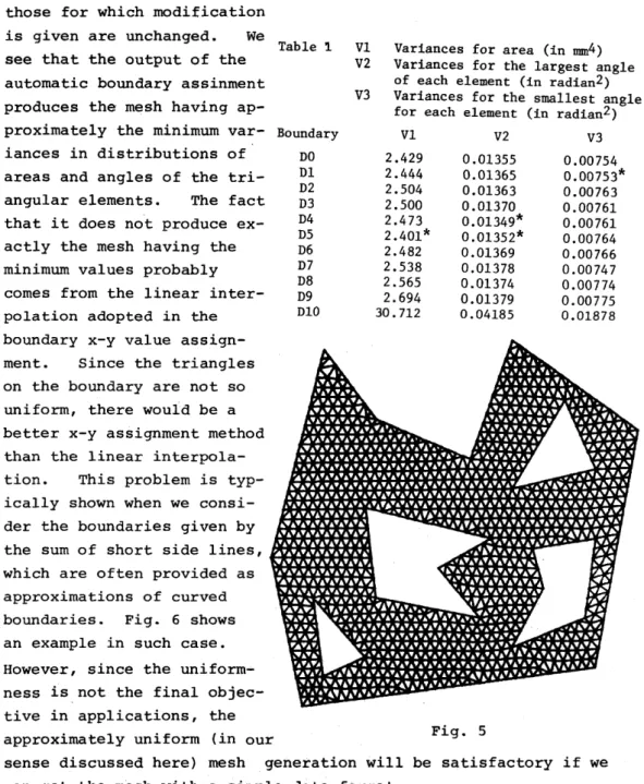
Fig.S shows an example in case the region has holes.

Fig.3 and Fig.5 show that the triangular element on the inner region are very uniform, but that the elements on the boundary are not so uniform respect to their areas and shapes.

In order to investi- gate how uniform meshes are realized, we calculate the variances in distributions of areas and angles of the whole triangular elements.

The output of the automatic boundary assignment are modified to a small extent as shown in Fig.2. The results obtained are shown in Table 1 together with the case of Fig.4 (=DIO). The results without modification are shown as DO. The modification gives the in- creases in their variances with a few exceptions, which are shown by

*

in the table.

The modification from Dl to D9 is rather small since the other partsof boundary than

~

J

i

Fig. 3

~

..

_{n~ ~}

~~l

,

~JlJ

J

Fig. 4

~

.30.

.L

'"

^lIo..

"V

" '?

too

...

~

~!\j ~~.

:-I~

I~

,,_ ::J

=~ ...

I

(7)

126

those for which modification is given are unchanged. We see that the output of the automatic boundary assinment produces the mesh having approximately the minimum variances in distributions of areas and angles of the triangular elements. The fact that i t does not produce exactly the mesh having the minimum values probably comes from the linear interpolation adopted in the boundary x-y value assignment. Since the triangles on the boundary are not so uniform, there would be a better x-y assignment method than the linear interpolation. This problem is typ- ically shown when we consi- der the boundaries given by the sum of short side lines, which are often provided as approximations of curved boundaries. Fig. 6 shows an example in such case.

However, since the uniformness is not the final objec- tive in applications, the approximately uniform (in our

Table 1 VI V2 V3 Boundary

DO D1 D2 D3 D4 D5 D6 D7 D8 D9 DI0

Variances for area (in mm4) Variances for the largest angle of each element (in radian2) Variances for the smallest angle for each element (in radian2)

VI V2 V3

2.429 0.01355 0.00754 2.444 0.01365 0.00753*

2.504 0.01363 0.00763 2.500 0.01370 0.00761 2.473 0.01349* 0.00761 2.401* 0.01352* 0.00764 2.482 0.01369 0.00766 2.538 0.01378 0.00747 2.565 0.01374 0.00774 2.694 0.01379 0.00775 30.712 0.04185 0.01878

Fig. 5

sense discussed here) mesh generation will be satisfactory if we can get the mesh with a simple data format.

(8)

Fig. 6

References

1. For example,

o.c.

Zienkiewicz and D.V. Phillips, Int. J. Num.

Meth. Eng.,

l

(1971) 519.

2. A.M. Winslow, J. Compo Phys. ~ (1967) 149.

3. K. Halbach and R.F. Holsinger, Particle Accelerators,2 (1976) 47.

4. K. Halbach, R.F. Holsinger, W.E. Jule and D.A. Swenson, Froc. of Proton Linear Accel. Conf., Chalk River, 1976.

5. R.S. Varga, Matrix Iterative Anal.ysis, Prentice Hall,1962.

(9)

128

Automatic Mesh Generation on a Polygonally Bounded Region