Business Cycles and Seasonal Cycles in Bangladesh

Business Cycles and Seasonal Cycles in Bangladesh

著者 Rahman Pk. Md. Motiur, Yamagata Tatsufumi

権利 Copyrights 日本貿易振興機構（ジェトロ）アジア

経済研究所 / Institute of Developing

Economies, Japan External Trade Organization (IDE‑JETRO) http://www.ide.go.jp

journal or

publication title

IDE Discussion Paper

volume 1

year 2004‑04‑01

URL http://hdl.handle.net/2344/203

INSTITUTE OF DEVELOPING ECONOMIES

Discussion Papers are preliminary materials circulated to stimulate discussions and critical comments

         

DISCUSSION PAPER No. 1

Business Cycles and Seasonal Cycles in Bangladesh

^*

Pk. Md. Motiur Rahman

^†

and Tatsufumi Yamagata

^‡

April 2004

Abstract

The empirical regularities of the Bangladesh business and seasonal cycles are documented in this study. Spectrums, seasonality, volatility, cyclicality, and persistence in the level and variance of macroeconomic variables in Bangladesh are explored using monthly and quarterly

macroeconomic series. Most of the features of U.S. and East-Southeast Asian business cycles are common to Bangladeshi business cycles; however, there are some differences. As is seen in the U.S. and European economies, seasonal cycles accentuate the features of business cycles in Bangladesh. To our surprise, the seasonal cycles in Bangladesh embody the features of business cycles in the U.S. and East-Southeast Asian economies more thoroughly than they do the

business cycles in Bangladesh

.

Keywords: business cycles, seasonal cycles, Bangladesh JEL classification: E32, O53

*

We would like to thank Sajjad Zohir for his useful comments. Mohammad Yunus helped us use econometric applications for this study. Karar Zunaid was an excellent research assistant.

† Professor, Institute of Statistical Research and Training, University of Dhaka.

‡ Director, Development Strategies Studies Group, Development Studies Center, IDE ([email protected]).

The Institute of Developing Economies (IDE) is a semigovernmental, nonpartisan, nonprofit research institute, founded in 1958. The Institute

merged with the Japan External Trade Organization (JETRO) on July 1, 1998.

  

The Institute conducts basic and comprehensive studies on economic and related affairs in all developing countries and regions, including Asia, Middle East, Africa, Latin America, Oceania, and East Europe.

The views expressed in this publication are those of the author(s). Publication does not imply endorsement by the Institute of Developing Economies of any of the views expressed.

INSTITUTE OF DEVELOPING ECONOMIES (IDE), JETRO 3-2-2, WAKABA,MIHAMA-KU,CHIBA-SHI

CHIBA 261-8545, JAPAN

©2004 by Institute of Developing Economies, JETRO

1. Introduction

A severe financial crisis hit East and Southeast Asian economies in 1997. No economy among those countries has completely recovered. The crisis reminded economists of the

importance of research on short-term macroeconomic fluctuations even for developing economies.

Because one of the foremost problems in any developing country has been considered to be raising the growth rate of the economy in order to escape the vicious circle of poverty, economists working for developing economies were more likely to study the long-run trends of macroeconomic variables rather than short-run fluctuations. However, we learned, as a result of the East-Southeast Asian financial crisis, that even when the growth potential of an economy is apparent, if great short-term turbulence strikes the economy, then the course of the growth path of the economy is seriously changed. In fact, endogenous growth models have a feature such that even if the turbulence takes place in the form of a temporary shock, the long-run growth trend of the economy may be affected (Aghion and Howitt, 1992; Rebelo, 1991; and Romer, 1986, among others). The effect of short-term fluctuations on the economy may be prolonged for a quite long period.

However, there have not been a sufficient number of comprehensive studies of the business cycles in Asian economies using modern time-series analysis techniques . The studies of Agénor, McDermott and Prasad (2000); Kim, Kose and Plummer (2000), and Yamagata (1998) are among the few that have been conducted. There are some studies focusing on necessary conditions to achieve rapid economic growth in Bangladesh (World Bank and Bangladesh Centre for Advanced Studies, 1998; World Bank, 1995, 1999); however, modern time-series analysis was rarely applied (Chowdhury, 1995; Rahman 2001; and Yunus, 1997, 2000, 2001). Moreover, most of the studies using time-series analyses examine long-term relationships among macroeconomic variables by estimating co-integrating vectors; they touch on short-run relations only incidentally.

Accordingly, the purpose of this study is to research empirical regularities in short-run economic fluctuations in Bangladesh. This study is expected to form “stylized facts” about the Bangladeshi economy. Theoretical works may use the findings of our study in the future to construct economic models that describe the mechanisms underlying the Bangladeshi economy. In this paper, we study the major macroeconomic variables of Bangladesh that are available and that have monthly frequencies from the beginning of the 1980s to the present. Those variables are industrial production, import, export, money supply (M1 and M2), wholesale price index (WPI, hereafter), consumers’ price index (CPI, hereafter), stock price index, and real wage.¹

In this study we focus on two kinds of short-term fluctuations, i.e., business cycles and

1 All the series cited are from the Monthly Bulletin of Statistics published by the Bangladesh Bureau of Statistics.

Obvious typos were cleaned. Adjustment of base years was made for industrial production.

seasonal cycles, which will be precisely defined in the next section. The business and seasonal cycles of the U.S. have been extensively studied; therefore, we use the U.S. economy as a benchmark in this study.

Key stylized facts about the U.S. business cycles as follows:² (1) Import and export are procyclical³ and more volatile than output.

(2) Monetary aggregates are procyclical and lead the cycle.

(3) Prices are less volatile than output and have been counter-cyclical since World War II.

(4) Stock price is very volatile and pro-cyclical; it leads the cycle.

(5) Hourly real wage is slightly pro-cyclical.

(6) All macroeconomic variables are serially correlated.

(7) Variance of inflation rate is serially and positively correlated.

These stylized facts are generally shared with developing countries with only a small number of exceptions (Agénor, McDermott and Prasad, 2000; Kim, Kose and Plummer, 2000; and Yamagata, 1998). Therefore, these features of the U.S. economy are meaningful as benchmarks for the investigation of the business cycles of the Bangladesh economy.

In addition, some of the features have direct and indirect policy implications. For example, the second feature (monetary aggregates) is sometimes referred to as supporting evidence for causality from money to production. The positive correlation between a current and past increase in money supply and a current increase in production is consistent with the hypothesis that monetary expansion causes an increase in production. It is known that a simple general equilibrium model introducing some price rigidity can reproduce the monetary aggregate feature, while one without price rigidity cannot (Cooley and Hansen, 1995). If prices are sticky, Keynesian demand management policies will be justified.

The feature (5) is consistent with an increasing returns model (Caballero and Lyons 1992;

Farmer, 1993; and Farmer and Guo, 1995). Real wage is regarded as a proxy for marginal labor productivity. A positive correlation between current productivity and output is referred to as procyclical productivity. If the aggregate production function of an economy exhibits constant returns to scale (or decreasing returns to scale), as long as output and factors of production change on the surface of the production function, the correlation between productivity and output must be non-positive. The observed procyclical productivity is consistent with increasing returns

2 These features are cited from Cooley and Prescott (1995), Kydland and Prescott (1990), Cooley and Hansen (1995), and Bollerslev (1986).

3 When a variable is positively correlated with output (or income), the variable is labeled “procyclical.” If the correlation is negative, the variable is labeled “counter-cyclical.” If a variable is not correlated with output, the variable is “acyclical.”

technology, though some other explanations are also possible.⁴ Increasing returns-to-scale technology is not harmonious with perfect competition. Either monopolistic power or externality must be accompanied for the segment of the production function exhibiting increasing returns to be seen as equilibrium. Whether monopolistic power or externality is applicable, market equilibrium is sub-optimal making active government policy justified.

Increasing returns-to-scale are known as a factor of sustainable long-term growth.

Romer (1986), which features increasing returns, is a pioneer of the endogenous growth theory, which led to the discussion of economic growth and development in the 1980s-90s. The procyclical-wage feature (5) is consistent with Romer’s model.

Second, seasonal cycles in the United States and other developed countries have been also extensively studied (Barsky and Miron, 1989; Beaulieu and Miron, 1992; and Miron, 1996), and the following features of the seasonal cycles have been found:

(8) Seasonal fluctuations are an important source of variation in macroeconomic quantity variables.

(9) Seasonal fluctuations are not applicable to prices. (This feature has been confirmed only in the U.S.)

(10) The seasonal components of money and real output are highly and positively correlated.

(11) The seasonal components of prices vary less than those of quantities (confirmed only in the U.S.).

(12) The seasonal components of labor productivity and industrial production are highly and positively correlated.

Notice that features (10) and (11) are the same as the stylized facts about the U.S. business cycles. Moreover, feature (12) is parallel to feature (5). In these ways, the characters of seasonal cycles mirror those of the business cycles in the U.S. economy (Miron, 1996).

The main conclusion of this study is that most of these features of the U. S. and

East-Southeast Asian business and seasonal cycles are common to the Bangladesh economy. The variance of inflation feature (7) is elaborated more in the final part of this study, and the mechanism of the evolution of the variance in inflation rates are analyzed with the Generalized Autoregressive Conditional Heteroskedasticity (GARCH) model.

4 Technology shocks and factor hoarding hypotheses are also consistent with the procyclical productivity, and they are more plausible hypotheses than increasing returns hypothesis. In fact, the feature (6) is consistent with factor hoarding hypothesis. For technology shocks, see Barro (1993). For factor hoarding, see Bils and Cho (1994), Burnside and Eichenbaum (1996), and Burnside, Eichenbaum and Rebelo (1993). For empirical research on returns to scale, see Basu (1996), Burnside (1996), Burnside, Eichenbaum and Rebelo (1995), Burnside and Yamagata (1998), and Yamagata (2000).

The remaining part of this paper is organized as follows. In the next section, the importance of fluctuation of different period of the cycle is studied with the spectral analysis. By estimating spectrum of log of monthly industrial production in Bangladesh, we will point out the importance of linear trends, business cycles, and seasonal cycles. In the third section, fluctuations in macroeconomic variables at the business cycle and higher frequencies are investigated. Features of the business cycles in Bangladesh are compared with the features of U.S. business cycles,

discussed above. The seasonal cycles are studied in the fourth section. Again, their features are compared with those of U.S. seasonal cycles. In the fifth section, serial correlation of variance in inflation rates and the rate of change in stock price are investigated. After seeing serial correlation of the variance in the rate of changes in WPI, CPI and stock price index, we estimate models of the variances with the GARCH model. The final section concludes.

2. Spectral Analysis of Industrial Production

It is known that a time series can be decomposed into fluctuations of different period of the cycle by the Fourier transformation. The estimated spectrum of each period of the cycle represents the importance of the fluctuations of the period. This technique is spectral analysis.⁵

The logarithm of the industrial production index in monthly frequencies in Bangladesh is shown in Figure 1 as an example. It is obvious that this series has time-trend and short-term fluctuations and that the period of the cycle is a year. Moreover, it is noticeable that there appears to be a long swing running through the sample period, which makes the time trend appear to be non-linear. In this way, a time series consists of fluctuations of various periods of the cycle.

The spectral analysis decomposes a time series into fluctuations of different periods of the cycle. Figure 2 shows the estimated spectrum for the log of monthly industrial production against the frequency of the cycle.⁶ In general, for most of macroeconomic time series, a linear time trend is important in terms of variation. Note that a linear trend can be interpreted to be the fluctuation of the period of the cycle of infinity (namely, its frequency is zero). This can be seen in Figure 2, where the lower the frequency of industrial production, the more important the fluctuation. The estimated spectrum decreases almost monotonically as the frequency increases. That is, fluctuations of longer period of the cycle are more important than those of shorter period in the series. This feature is common to all variables in this study; however, their spectrums are not displayed to save space.

Once a time trend is suppressed from the series, short-term fluctuations become

5 See Hamilton [1994] and Harvey [1993] for the spectral analysis.

6 Precisely speaking, this is the ratio of the frequency to the circular constant,

π

. In other words, the unit of the axis is

π

.

conspicuous. In fact, there are various methods for de-trending. Each method has its own operator, or “filter,” with which the original series is transformed into the de-trended series.

First-difference Filter

First, let us use the first-difference filter in order to de-trend the industrial production series. The first-difference in a logged variable is a proxy for the growth rate of the original variable. It is a familiar indicator used to see the short-run fluctuations of a time series. Figure 3 shows the estimated spectrum of the logged and first-differenced industrial production. As a result of the de-trending, five outstanding humps appear in Figure 3. The hump at shows the importance of fluctuations of the period for a cycle of twelve

6•

1 . 0

7, i.e., one year. In the same way, the following four humps correspond to fluctuations whose period of the cycle are 6, 4, 3, and around 2.4, respectively.⁸ The fluctuations of a one-year period of the cycle are denoted as “seasonal cycles.” It is seen in Figure 3, seasonal cycles are important components of log of industrial production in the monthly frequency.

However, the first-difference filter is known to over accentuate higher-frequency fluctuations (Stock and Watson, 1999, Fig. 2.4). Another range of important lower-frequency fluctuations is repressed, which is hardly discernible in Figure 3. According to the convention of modern business-cycle literature, those important lower-frequency fluctuations are called “business cycle,” and the period of the cycle is approximately three to five years (Cooley and Prescott, 1995, pp. 27-28). In fact, there is a tiny hump at the frequency of 0.03, which corresponds to the period of the cycle at five and half years.

Year-to-year First-difference Filter

Taking a year-to-year growth rate⁹ instead of a month-to-month growth rate, suppresses not only the time trend but also seasonal fluctuations. Figure 4 exhibits the estimated spectrum for the year-to-year growth rate of industrial production. Notice that as is the case in Figure 2, the fluctuations of the lower frequencies of the cycle turn are more important than those of higher frequencies as a whole.¹⁰ In addition, note that in Figure 4 the estimated spectrum becomes a

7 212=0.166^•.

8 The corresponding relative frequencies of the cycle are 0.33^•, 0.5, 0.66^•, and 0.825.

9 The year-to-year growth rate is approximated by

ln x

_t

− ln x

_t−12.

10 Though the spectrum of the linear trend whose frequency of the cycle is exactly zero looks high, that is because of smoothing made for the estimated spectrum to be a consistent estimator of the population spectrum. In fact, the linear trend is supposed to be repressed with the year-to-year difference filter ( see Hamilton, 1994).

trough at all of the frequencies where the outstanding five humps are seen in Figure 3. The fluctuations of the business-cycle frequency become one of the most important fluctuations in terms of the variance.

Hodrick-Prescott Filter

Using a first-difference filter cannot eliminate the very long waves that are incorporated in a time series. Hodrick and Prescott (1997) invented a simple and practical filter that can suppress low frequency cycles. The Hodrick-Prescott filter (hereafter, the H-P filter) is defined as follows.

Suppose a time series

x

_t is divided into growth component,

x

_t^g, and cyclical component,

x

_t^c:

c t g t

t

x x

x = +

. (1)

Then, the H-P filtering problem is to choose the growth component, , to minimize the following function:

g

x

t

( ) _∑ [ ( ) ( )

∑

= + −

=

−

−

− +



 

 

T

t

g t g t g t g t T

t c

t

x x x x

x

1

2 1 1

1

2

λ ]

^{, (2)}

where

T

is the terminal period, and

λ

is a constant which is set according to the frequency of the data set.¹¹ If the value of

λ

was zero and the second term vanishes, , would solve

the problem, and the H-P filter would return the original series as the growth component, ’s.

On the other hand, the second term is minimized when is the same for any

t

. Therefore, if the first term did not exist, the H-P filter would return a linear trend as the growth component.

That is, the first term yields a growth component that is close to the value of the original series, while the second term makes the growth component smooth.

t x

_t^c

= 0 , ∀

g

x

t

g t g

t

x

x −

₋₁

λ

is a weight of the second term relative to the first term.

If

λ

is properly chosen, the H-P filter extracts fluctuations for which the period of the cycle is eight years or shorter.¹² Figure 5 displays the estimated spectrum for the H-P filtered log of industrial production. As was shown in Figure 3, there are humps in the estimated spectrum at the frequencies of around 0.167, 0.333, 0.500, 0.667 and 0.825, which correspond to the periods for 12, 6, 4, 3, and 2.4, respectively. However, at this time, in addition to those humps, there is a moderate

11 For annual, quarterly and monthly series (100, 1600, and 14,400 respectively), are conventionally used. However, Burnside (2000) argues that the value of 129,000 is more appropriate for monthly series.

12 A comparison of the first difference filter and H-P filter is provided by Stock and Watson (1999, Fig. 2.4).

hump at the frequency of around 0.05, which corresponds to the period of 40 months. This hump represents the importance of the fluctuations of the business-cycle frequencies. Though the height of this hump is lower than those of the periods for twelve and six, it is higher than the other humps.¹³ This implies that cycles whose frequencies are less than that of the seasonal cycle are important in the industrial production series in Bangladesh.

Conventionally, seasonally-adjusted and H-P filtered fluctuations are called “business cycles” in the modern business-cycle literature. Hereafter we follow this convention, and refer to H-P filtered fluctuations as the business cycles. In the next section, the business cycles, i.e., seasonally-adjusted and H-P filtered fluctuations of macroeconomic series, are extensively studied.

In the section four, the seasonal cycles are extensively studied in turn, and compared with the business cycles.

3. Business Cycles in Bangladesh

In this section, empirical regularities of the business cycles in Bangladesh are given. The features of the Bangladesh business cycles will be compared with those of the U.S. and

East-Southeast Asian business cycles that were shown in the introduction.

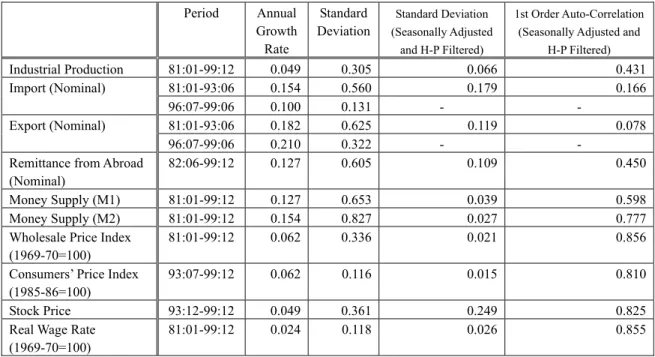
Basic statistics for macroeconomic variables in Bangladesh, which are available in monthly frequency, are shown in Table 1 (see Appendix for details of the data.). However, we use not only monthly series but also quarterly series that are transformed with the monthly series, because (a) most of research on U.S. business cycles uses quarterly data and because (b) we want to compare the Bangladesh business cycles with the U.S. business cycles. Table 2 displays basic statistics in quarterly series.

In the next section, we explore the empirical regularities for the stationarity, volatility, persistence, and cyclicality of the series.

Stationarity: Time trend

In general, stationarity relates to constancy of moments of a series over time. Here, we focus on stationarity of the first moment, namely mean, of macroeconomic variables, because the mean of usual macro quantity and price series are not constant over time (Cooley and Prescott, 1995;

Stock and Watson, 1999, among others). And if they are non-stationary variable, e.g., a

random-walk series, they are solely determined by the stochastic disturbances and are unpredictable.

Therefore, it is important to know whether or not a series is stationary.

13 Here the conventional value of

λ

of 14400 is used for H-P filtering. However, if a greater value is used according to the suggestion of Burnside (2000), the growth components will be smoother and the spectrum at lower frequencies will be accentuated more.

All the variables displayed in Table 1 are non-stationary in the sense that their logarithms have time trends. That is, the first moments of the variables are not constant over time. In addition, their annual growth rates are significant, and in particular, the growth rates of import, export and remittance are very high by any standard, although they have nominal values and include changes in their prices.¹⁴

The Augmented Dickey-Fuller (ADF) Test is used to examine whether the trend of a time series is stochastic and has the random-walk property or is deterministic. According to the ADF test with twelve period lags, the level of all variables is non-stationary, and most of the variables are integrated of order one, I

( )

1 .¹⁵

Volatility: Variance

The monthly standard deviation of logged macroeconomic variables is displayed in the third column of Table 1. Since they are logged series, the unit of the standard deviation is a percentage. In general, rapidly growing series show high variation because the trend part

contributes to the high variation. Therefore, de-trended and seasonally adjusted series are used in order to analyze business cycle fluctuations in Bangladesh in this section.

The standard deviation of industrial production in quarterly frequency is 4.2%. Since the standard deviation of industrial production in the manufacturing industry in the United States for 1981:1Q-99:1Q is 1.1%, and the same statistic for Japan for 1981:1Q-98:4Q is 3.4%, industrial production in Bangladesh is more volatile than that in the United States and Japan. Other variables in Bangladesh are also more volatile than their U.S. counterparts. For example, the standard deviation of log import and export in Bangladesh is 13.2% and 9.0%, while those of the United States for 1954:1Q-91:2Q are 4.9% and 5.5%, respectively. The same statistics of M1, M2, CPI and real wage rate in the United States for the same period are 1.5%, 1.5%, 1.4%, and 1.5%, respectively, (Cooley and Prescott, 1995; Cooley and Hansen, 1995; and Kydland, 1995). In Bangladesh, all these variables are more volatile (Table 2). Kim, Kose and Plummer (2000) and Yamagata (1998) point out that macroeconomic variables for the East-Southeast Asian developing economies are more volatile than those of developed countries. Bangladesh shares the same feature of high volatility with East-Southeast Asian developing economies.

For Bangladesh, the tendency of relative volatility of macroeconomic variables relative to output is similar to that of the United States. Since quarterly GNP series are not available in

14 Monthly import and export series are not available for 1993:07-1996:06.

15 I(1) implies that the level of a logged variable is non-stationary while its first difference is stationary. The log difference of import (1996:07-1999:06), export (1996:07-1999:06), M2, CPI and stock price with twelve-period lags without trend are not stationary. However, all of them are stationary with four or smaller period lags. The results of the ADF test are available from the authors upon request.

Bangladesh, we use industrial production as an indicator of production in Bangladesh. Import, export, and remittance are more volatile than output. Monetary aggregates, prices, and real wage are less volatile than output. Stock price is as five times as volatile as industrial production, which suggests that there is a high instability in the stock market in Bangladesh.

Persistence: Serial Correlation

Macroeconomic variables tend to be serially correlated in the U.S. and European and East Asian countries even after time trends are eliminated (Cooley and Prescott, 1995; Stock and Watson, 1999; Kim, Kose and Plummer, 2000; and Yamagata, 1998). This finding suggests that the effects of a shock do not terminate instantaneously and that those effects continue for a certain period.

Such gradual transmission of a shock may be due to capital accumulation, adjustment costs, a delay in recognition, etc. The effects of shocks in macroeconomic variables tend to be persistent in Bangladesh, too(Table 2). However, there are important exceptions. Import and export are not highly serially correlated. Their estimated first order auto-correlation coefficients are low and statistically insignificant. This tendency is confirmed by the monthly import and export series (Table 1). The movement of import and export seems to be dominated by transient shocks and seasonal cycles, so that only small portion is affected by past shocks in Bangladesh.

Cyclicality: Correlation with Production

Cyclicality is a core concept of business-cycle research. A procyclical variable is positively correlated with production and income, while a counter-cyclical variable is negatively correlated. A variable without a correlation with production is called “acyclical.” Correlation with GNP is a major concern for economists when they think of the mechanism of macroeconomic fluctuation.

Quarterly GNP series are not available in Bangladesh. Therefore, we use industrial production, which covers mining and quarrying, manufacturing and electricity generation, in place of GNP, in order to analyze cyclicality of macroeconomic variables in Bangladesh. Industrial production is often used as a benchmark of research in seasonal cycles in the U.S. (Miron, 1996, among others), since industrial production series in monthly frequency are available for many countries, and industrial production series reflect fluctuations in production for the whole economy.

In this sub-section, (1) cyclicality of macroeconomic variables, which is the correlation between industrial production and current variable, and (2) lead-and-lag structure of macroeconomic variables, which is the correlation between current industrial production and past and future values of the other macroeconomic variables, are examined. The correlation coefficient between current industrial production and macroeconomic variables at time

t + i (

i =−4,−3,K,0,K4

)

and its standard error in parentheses by the OLS are shown in Table 2, columns 3-11.

The first row of Table 2 shows the correlation between current industrial production and a past or future value of it, which demonstrates the persistence of shocks in industrial production.

These correlation coefficients are called by autocorrelation of industrial production. As mentioned in the previous sub-section, the autocorrelation with a one-quarter lag is positive and statistically significant.

In Table 2, columns 2-10 portray the cyclical relations between industrial production and other macroeconomic variables. First, the correlation coefficient between current import and industrial production is 0.16, which is not significantly different from zero. That is, import is weakly procyclical. Positive correlation between import and production is observed unanimously both across country and over time in many countries in the world. The statistic shows that

Bangladesh barely shares the same tendency. The correlation coefficient between current industrial production and import one-quarter ahead is also moderately high, 0.26. The right half of the second row of Table 2 shows that current industrial production tends to be correlated with future import, and that the positive correlation between current industrial production and import one year ahead is statistically significant. Industrial production leads import, probably because when many manufactured goods are supplied to the market, import increases not only in the current period but also for a year ahead. Meanwhile, export and remittance are almost acyclical in the business-cycle frequencies. It seems that export and remittance are not affected by the business cycles in the Bangladesh economy, but are dependent on the business cycles of the country that imports goods and labor from Bangladesh.

Monetary aggregates are significantly procyclical. While the correlation between current monetary aggregates and industrial production is moderate, it is statistically significant. Moreover, both monetary aggregates lead production. For both M1 and M2, the correlation between current industrial production and the value one quarter before is greater than 0.30, while the same statistics with the monetary aggregates two quarters before are also moderately high and statistically significant. This feature is common to the U.S. and some East-Southeast Asian economies.¹⁶ While this observation is consistent with causality from money to output, it is harmonious with the endogenous money hypothesis as well. The endogenous money hypothesis argues that money supply is endogenously determined and responds more quickly than output (King and Plosser, 1984, among others). Serious debates about causality between money and output have arisen among members of the U.S. academic community, and since because it has been found that money leads output for the Bangladeshi economy, the same question about causality between money and production is applicable to the Bangladeshi economy.

Both wholesale price and consumers’ price are very weakly procyclical. If the demand

16 Monetary aggregates lead GDP with one-year lag in the United States, Hong Kong, South Korea, Singapore and Taiwan (Yamagata, 1998).

shocks dominated the supply shocks, price would be positively correlated with production, because demand shocks in price stimulate production. If the supply shocks dominate, the correlation between price and output is negative, because abundant supply of goods lowers prices. Therefore, it seems that the effects of the demand and supply shocks offset each other and result in an

insignificant correlation between price and output in the Bangladeshi economy.

Stock price is negatively correlated and does not have any statistically significant

correlation with industrial production within the range of leads and lags of four quarters. Since the standard error of each correlation coefficient is so great, even with the moderately high value of correlation coefficient, the null hypothesis that the correlation coefficient is zero is not rejected for the stock price. In the U.S. economy, stock price is procyclical, it leads production, and an increase in stock price is a leading indicator for predicting an increase in production. Stock price in

Bangladesh does not play such a role probably because the scale of stock market is not as great as in the United States. Chowdhury (1995) reaches the same conclusion, finding little causality from lagged stock price to current money supply for the Bangladeshi economy between January 1982 and May 1995.

Real wage rate is almost acyclical. In the next section we will show that the positive and significant correlation between real wage and production appears in the seasonal cycles. However, the positive correlation between real wage and production is not apparent in the business-cycle frequency in Bangladesh.

So far, most of the benchmark features of business cycles discussed in points 1-6 in the introduction are applicable to Bangladeshi business cycles as well. This implies that a similar mechanism of business cycles works in Bangladesh and in the economies of the U.S. and East-Southeast Asian countries.

The economic models that are applicable to the economies of the U.S. and East-Southeast Asian countries are likely to fit the Bangladeshi business cycles well. However, there are some important differences from the benchmark features of business cycles, which researchers should keep in mind: import and export are not strongly procyclical; prices are acyclical; stock price is acyclical and does not lead the cycle; real wage is almost acyclical; and serial correlation of import and export are not strong in Bangladesh.

4. Seasonal Cycles in Bangladesh

Seasonal components tend to be eliminated without due consideration when a macro economy is studied. People prefer seasonally adjusted series to unadjusted series without knowing what is contained in the seasonal components. Barskey and Miron (1989), Beaulieu and Miron (1992), and Miron (1996) found that seasonal components and business-cycle fluctuations had

many features in common. In particular, they found that there is a remarkable correlation between the seasonal components of production and those of macroeconomic variables, which were similar to the ones found with the seasonally-adjusted and de-trended production and macroeconomic variables.

That is, they found important cyclicality in the seasonal components of macroeconomic variables.

Therefore, they called the seasonal components “seasonal cycles.” We use their terminology.

In this paper, we follow Miron (1996) and seasonal cycles are defined as the predicted value resulting from regression with seasonal dummies used as regressors. In this section, the original monthly series are used, because monthly series have richer information than quarterly series that are made of monthly series.

Significance of Seasonal Cycles

First, we show that the seasonal components are quite important in the short-term

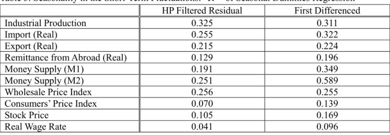
fluctuations of quantity series and monetary aggregates in Bangladesh, as was found for the U.S. and European economies (Beaulieu and Miron, 1992). Table 3 displays the importance of the seasonal cycles in the short-term fluctuations of macroeconomic variables in Bangladesh. As the short-term fluctuations, not only the H-P filtered series but also first differenced series (a proxy for a growth rate), are used. The first differenced series is used in order to check the sensitivity of the results to de-trending methods. In order to examine the importance of the seasonal components, we regress either the H-P filtered series or the first differenced series on eleven monthly dummies and an intercept, and define the predicted value as the seasonal component. The coefficient of determination of the regression,

R

², is shown in Table 3.

In general, the seasonal components are important in the short-term fluctuation of quantity series in Bangladesh. The seasonal components explain approximately 33% of the total variation of the H-P filtered industrial production. As for import, approximately 25% is explained by the seasonal components, while approximately 20% is explained for export. However, seasonal fluctuations are not as important for remittance from abroad as for industrial production, import and export. About 13% of the H-P filtered remittance is explained with monthly dummies. The seasonal components are as important in the first differenced quantity series as in the H-P filtered quantity series. The coefficients of determination for the first differenced series are as great as for H-P filtered series in the second column of Table 3.

Seasonal components are moderately important in H-P filtered monetary aggregates.

Meanwhile, they are very important in the first differenced monetary aggregates. The coefficient of determination of the monthly dummy regression is over 0.3 for M1, while the same coefficient is almost 0.6 for M2. By contrast, seasonal components are not as important in price series as in quantity series in Bangladesh. This feature is shared with the U.S. and European economies.

With the exception of WPI, the coefficients of determination of the monthly dummy regression with

both H-P filtered and first differenced price series (i.e., CPI, stock price, and real wage rate) are smaller than 0.2.

Relative Volatility

The pattern of relative volatility of macroeconomic variables to industrial production in business-cycle frequencies, which is seen in the second column of Table 2, is almost exactly the same as that of the seasonal cycles in Bangladesh. Figures 6-11 compare the seasonal components of industrial production with those of other variables. There are three findings to be mentioned concerning relative volatility among seasonal components. First, the seasonal components of import and export are more variable than those of industrial production as (Figure 6). Remember that the components of import and export in business-cycle frequencies are more variable than that of industrial production (Table 2). Import and export are more variable than industrial production in not only the business cycle but also seasonal cycle frequency. Second, the seasonal components of price indices except stock price (i.e., WPI; CPI, and real wage) are less variable than those of industrial production (Figures 9 and 11). Third, the seasonal components of stock price are very volatile as are the H-P filtered series (Figure 10).

Seasonal Co-movement

The pattern of seasonal co-movements is also similar to that of the business cycle

frequencies. In Table 4, the correlation coefficients between the seasonal components of industrial production and other variables are displayed. The seasonal components of import and export are highly correlated with those of industrial production. The correlation coefficients of the seasonal components of industrial production and those of import and export are 0.60 and 0.72, respectively.

There is a jump in import in June that is not followed by a comparable increase in industrial production (Figure 6). However, import and industrial production behave similar in the other months. The seasonal components of export move around those of industrial production, too, though the correlation coefficient between seasonal components of export and those of industrial production is not significantly different from zero in the statistical sense.

Remittance and monetary aggregates also follow industrial production very well in terms of seasonal fluctuation (Figures 7 and 8). Those of monetary aggregates look more similar to those of industrial production than remittance. The correlation coefficients of the seasonal components of industrial production and those of remittance, M1 and M2 are 0.62, 0.49, and 0.72. The only discrepancies between monetary aggregates and industrial production are the following: (1) the seasonal components of the monetary aggregates do not follow an increase in those of industrial production in January, and (2) the monetary aggregates do not follow decreases in industrial production in May and July.

The correlation coefficients between the seasonal components of wholesale price and consumers’ price indices and those of industrial production are negative, though they are not statistically significant (Figure 9). Note that prices are likely to be counter-cyclical in U.S.

business-cycle frequencies. Thus, the pattern of correlation between prices and production for seasonal frequency in Bangladesh is closer to that of U.S. business cycles than to that of Bangladeshi business cycles.

By contrast, the seasonal components of real wage are positively and significantly correlated with those of industrial production (Table 4 and Figure 11). This fact is remarkable because the correlation between real wage and industrial production in business cycle frequencies is not so high (Table 2). As the comparison of the pattern of correlation between prices and

production, the cyclicality of real wage in terms of seasonal cycles in Bangladesh is closer to that of U.S. business cycles than that of Bangladeshi business cycles. Cyclical wage suggests that labor productivity is highly procyclical at seasonal frequency in Bangladesh. Since labor has a nature of quasi-capital, the rewards for labor need not fluctuate as much as the marginal product does (Oi, 1962). It is remarkable, however, that even though the change in real wage according to productivity is likely to be mitigated, the procyclical nature remains in real wage series in Bangladesh.

Lastly, it is noticeable that the correlation coefficient between the seasonal components of stock price and those of industrial production is moderately positive (Figure 10).

In sum, there are two key findings: (i) seasonal components are important in quantity series and monetary aggregates, and (ii) the features of seasonal cycles mirror those of business cycles. The similarities between them are as follows: (ii-a) import and export are more variable than industrial production; (ii-b) price indices, except for stock price, are less variable than industrial production: (ii-c) import, export, M1 and M2 are positively correlated with industrial production.

However, there are remarkable differences such as (a) a high correlation between remittance and industrial production; (b) a more strongly negative correlation between general price indicators (i.e., WPI and CPI, and industrial production); and (c) a positive and significant correlation between real wage and industrial production. These three differences between the features of seasonal cycles and those of business cycles in Bangladesh exactly coincide with the differences between the features of Bangladeshi business cycles and those of U.S. business cycles. Hence, the seasonal cycles in Bangladesh embody the features of U.S. business cycles more exactly than the business cycles in Bangladesh.

5. Auto-regressive Conditional Heteroskedasticity in Price Indices

So far, when we study serial correlation, we have focused at the level of macroeconomic variables. However, serial correlation may also take place in terms of a second moment, e.g., variance. That is, the population variance of a macroeconomic variable may be auto-correlated.

In particular, price variables (i.e., inflation rates, and rates of change of stock price, land price, exchange rate, etc.) are known to become very volatile once great shocks hit the economy, and such volatility tends to last for a certain time period. Therefore, price series are more likely to have this nature than quantity series.

There are estimation methods to handle the auto-regressive nature of variance. Engle (1982) pioneered this field of research, and introduced the Auto-regressive Conditional

Heteroskedasticity (ARCH) model. Bollerslev (1986) generalized Engle’s method and proposed the Generalized ARCH (GARCH) model. In this section, we study the auto-regressive nature of the variance of three price series in Bangladesh (WPI, CPI, and stock price).

Auto-correlation in the Squared Inflation Rate

Engle [1982] and Bollerslev [1986] found the variances of inflation rates and the rate of change in stock price were serially correlated in the U.K. and U.S., respectively. In fact, they are serially correlated in Bangladesh, too. Table 5 displays three statistics concerning auto-correlation, for auto-correlation coefficient (AC), partial auto-correlation coefficient (PAC), and Ljung-Box Q-statistics of the squared log-differenced price series. The auto-correlation coefficient is defined as follows:

( )( )

( )

∑ ∑

= +

= −

−

−

= _T −

t t

T k

t t t k

k x x

x x x r x

1

2

1 , (3)

where

T

is the sample size and

k

is the number of lags. The partial auto-correlation coefficient is the same as the ordinary partial correlation coefficient that is derived from determining the multiple regression of the current variable on lagged variables. The Ljung-Box

Q

-statistics are test statistics for the null hypothesis that there is no auto-correlation up to order

k

:

( ) ∑

=

−

+

=

^k

j j

j T T r

T Q

1 2

2

. (4)

The Ljung-Box

Q

-statistics are asymptotically distributed as a

χ

².

Table 5 shows auto-regressive nature of the variance of log difference in WPI, CPI, and stock price. The

p

-value of Q-statistics is given in the next column to that of Q-statistics. The first-order auto-correlation coefficient of WPI is positive and significant. And, this positive first-order auto-correlation is great enough for the null hypothesis of no auto-correlation with twelve lags to be rejected. The first order auto-correlation coefficient of CPI is also high, 0.389, and

statistically significant. However, it is not as significant as that of WPI so that the null hypothesis of no auto-correlation with twelve lags is accepted. Stock price exhibits an interesting pattern of auto-correlation in the squared rate of change. Its first order auto-correlation is not statistically significant, while the auto-correlation coefficients with four and five lags are both positive and significant. As a result, the null hypothesis of no auto-correlation with twelve lags is rejected.

GARCH Estimation

The three price indicators have their own patterns of auto-correlation in the squared rate of change. We analyze the auto-correlation in the squared rate of change in the three price indicators with the GARCH model. A GARCH model takes the following form:

t t

t

p u

p = + ∆ +

∆ ln β

₀

β

₁

ln

₋₁ , (5)

2 1 2

1

2

= +

_t−

+

_t−

t

ω α u γσ

σ

, (6)

where , and are a price, the disturbance, and the one-period ahead forecast variance at time

t

based on information up to time

t-1, respectively

. The first order auto-correlation in the logarithm of the price is assumed. ∆ is the differencing operator. The definition of is

p

t

u

_t

σ

_t²

2

σ

t

(

1

)

2

2 ≡ _t Ω_t−

t Eu

σ

, (7)

where

Ω

_t−1 is the information set at

t-1

. Let’s assume that

u

_t² follows ARMA(1,1):

( )

²_{1 1}

2

= + +

_t−

+

_t

−

_t−

t

u v v

u ω α γ γ

, (8)

where . Eq. (6) is derived from this assumption. Since the squared rate of change of stock price exhibits a complicated auto-correlation structure, a combination of auto-regression and moving average may help explain the movement of the squared rate of change of stock price.

When Engle (1982) introduced the ARCH model, the squared disturbance was assumed to follow the AR(1) process and neglected the moving average part (i.e.,

2 2

t t

t

u

v ≡ − σ

= 0

γ

) was assumed. Subsequently, Bollerslev (1986) introduced the moving average part, and eq. (8) is called the GARCH(1,1) model.

< 1 + γ

α

is required for

u

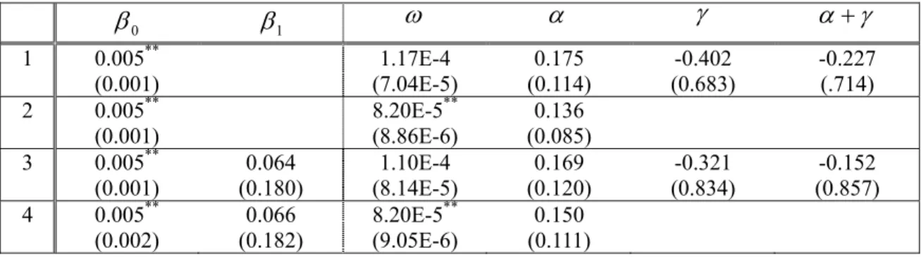
_t² to be stationary.

The estimation results of the GARCH model for the three price indicators are shown in Tables 6-8. The coefficient of the auto-regression term of eq. (5),

β

₁, is assumed to be zero for the benchmark model, but it is estimated for the general model. The estimation results with WPI

show that the ARCH part, which is represented by

α

, is positive and significant in the variance equation, eq. (6), while the GARCH part, which is represented by

γ

, is not statistically significant, whether or not the auto-regression term is added to the level equation, eq. (5). The ARCH

coefficient is between 0.3 and 0.5, so that the effect of the shocks is short-lived. The behavior of variance of WPI in Bangladesh is described as an auto-regressive model.

The GARCH model does not provide a good explanation the variance of the inflation rate in terms of CPI. Whether or not the past inflation rate is added to the level equation, both the ARCH and GARCH parts are statistically insignificant. The variance of CPI in Bangladesh seems to follow neither an auto-regression nor a moving average, even though it is serially correlated (Table 5).

On the other hand, the variance of the rate of change in stock price fits the GARCH model very well. Regardless of the level of the equation, both the ARCH and GARCH terms are positive and statistically significant. The autoregressive-moving-average model explains the serial

correlation of the variance in stock price. Moreover, the estimated

α

+

γ

is greater than unity in all estimations. If the auto-regression is added to the level equation, even the alternative hypothesis that

α

+

γ

is greater than unity is accepted at a 95% level of significance. Those results suggest that the variance of the rate of change in stock price is a unit root process. That is, the variance of the rate of change in stock price is unpredictable.

6. Concluding Remarks

In this study we documented empirical regularities of the short-term fluctuations in the Bangladeshi macro economy. Basically, those regularities regarding business cycles are similar to what are found in the economies of the U.S. and East-Southeast Asian countries. Import and export are highly volatile.

ƒ Monetary aggregates are procyclical and lead the cycle.

ƒ Prices are less volatile than output, while stock price is very volatile.

ƒ Most of the macroeconomic series are serially and positively correlated.

ƒ The variance of the rates of change in WPI, CPI and stock price is serially correlated.

However, there are some deviations from the “stylized facts” of the U.S. business cycles.

ƒ Wholesale and consumers’ price indices and stock price are almost acyclical.

ƒ Import and export are not strongly procyclical and not highly auto-correlated.

In sum, the feature of U.S. business cycles from (1) through (7), as indicated in Introduction, are applicable to the Bangladeshi economy with a limited number of exceptions.

Seasonal cycles in Bangladesh have the same features as those of the United States. As in the case of U. S. seasonal cycles, seasonal components are important parts of the short-term

fluctuations especially for quantity series and monetary aggregates. The features of seasonal cycles tend to accentuate those of the business cycles. For example, the seasonal components of monetary aggregates are highly and positively correlated with those of industrial production, while the

seasonal components of prices except stock price are less volatile than those of quantities.

Moreover, the seasonal components of real wage are highly procyclical. As a result, the features of the seasonal cycles in the U.S. and other developed countries, points 8-12 in the introduction, are applicable to the seasonal cycles in Bangladesh. It is remarkable that the features of U.S. business cycles that are not mimicked by those of Bangladeshi business cycles are embodied by seasonal cycles in Bangladesh. Specifically, the seasonal components of import, export, stock price and real wage are positively correlated with those of industrial production, while the seasonal components of WPI and CPI are both negatively correlated with those of industrial production.

In addition, the serial correlation of the variance of the rate of change in price indicators was studied with the GARCH model, and the variances of WPI, CPI, and stock price are all serially correlated. The variance of WPI follows the AR(1) model, while that of stock price follows ARMA(1,1). In variance, the AR model is called the ARCH model, while in variance the ARMA model is called the GARCH model. Neither the AR nor the MA model explains the serial correlation of variance in CPI.

A general conclusion is that as far as short-term fluctuations are concerned, the mechanism controlling the Bangladeshi economy does not seem to be very different from that for the

economies of the U.S. and East-Southeast Asian countries. That is

1) Production, other quantity series, and money almost synchronize.

2) Stock price is very volatile, and, export and import, production and general price indicators follow stock price in order in terms of volatility.

3) Quantity series and monetary aggregates contain great seasonal components, while price indicators do not.

4) The seasonal cycles of macroeconomic series in Bangladesh embody the features of U.S. and East-Southeast Asian business cycles more thoroughly than do the business cycles in Bangladesh.

5) Variances of price indicators are likely to be serially correlated.

It is expected that the empirical regularities found in this study will be building blocks for constructing structural models of the Bangladeshi economy and developing appropriate macro stabilization policy for the economy.

References

Agénor, McDermott and Prasad 2000 : Pierre-Richard Agénor, C. John McDermott, and Eswar S.

Prasad, “Macroeconomic Fluctuations in Developing Countries: Some Stylized Facts,”

World Bank Economic Review, Vol. 14, No. 2, May, pp. 251-285.

Aghion and Howitt 1992 : Philippe Aghion and Peter Howitt, “A Model of Growth through Creative Destruction,” Econometrica, Vol. 60, No. 2, March, pp. 323-351.

Barro 1993 : Robert J. Barro, Macroeconomics, Fourth Edition. John Wiley & Sons, Inc., New York, USA.

Barskey and Miron 1989 : Robert B. Barskey and Jeffrey A. Miron, “The Seasonal Cycle and the Business Cycle,” Journal of Political Economy, Vol. 97, No. 3, June, pp. 503-534.

Basu 1996 : Susanto Basu, “Procyclical Productivity: Increasing Returns or Cyclical Utilization?”

Quarterly Journal of Economics, Vol. 111, Issue 3, August, pp. 719-751.

Beaulieu and Miron 1992 : J. Joseph Beaulieu and Jeffrey A. Miron, “A Cross Country Comparison of Seasonal Cycles and Business Cycles,” Economic Journal, Vol. 102, No. 413, July, pp.

772-788.

Bils and Cho 1994 : Mark Bils and Jang-Ok Cho, “Cyclical Factor Utilization,” Journal of Monetary Economics, Vol. 33, No. 2, April, pp. 319-354.

Bollerslev 1986 : Tim Bollerslev, “Generalized Autoregressive Conditional Heteroskedasticity,”

Journal of Econometrics, Vol. 31, No. 3, April, pp. 307-327.

Burnside 1996 : Craig Burnside, “Production Function Regressions, Returns to Scale, and Externalities,” Journal of Monetary Economics, Vol. 37, No. 1, April, pp. 177-201.

Burnside 2000 : Craig Burnside, “Some Facts about the HP Filter,” mimeographed, World Bank, Washington, D.C., USA.

Burnside and Eichenbaum 1996 : Craig Burnside and Martin Eichenbaum, “Factor-Hoarding and the Propagation of Business-Cycle Shocks,” American Economic Review, Vol. 86, No. 5, December, pp. 1154-1174.

Burnside, Eichenbaum and Rebelo 1993 : Craig Burnside, Martin Eichenbaum and Sergio Rebelo,

“Labor Hoarding and the Business Cycle,” Journal of Political Economy, Vol. 101, No. 2, April, pp. 245-273.

Burnside, Eichenbaum and Rebelo 1995 : Craig Burnside, Martin Eichenbaum and Sergio Rebelo,

“Capital Utilization and Returns to Scale,” in Ben S. Bernanke and Julio J. Rotemberg (eds.), NBER Macroeconomics Annual 1995, MIT Press, Cambridge, USA, pp. 67-110.

Burnside and Yamagata 1998 : Craig Burnside and Tatsufumi Yamagata, “Cyclical Factor Utilization and Returns to Scale in East Asian Manufacturing,” a paper presented at the winter meeting of the Korea International Economic Association held at Korea University, Seoul

on December 12, 1998.

Caballero and Lyons 1992 : Ricardo J. Caballero and Richard K. Lyons, “External Effects in U. S.

Procyclical Productivity,” Journal of Monetary Economics, Vol. 29, No. 2, April, pp.

209-225.

Chowdhury 1995 : A. R. Chowdhury, “Is the Dhaka Stock Exchange Informationally Efficient?”

Bangladesh Development Studies, Vol. 23, Nos. 1&2, pp. 89-104.

Cooley and Hansen 1995 : Thomas F. Cooley and Gary D. Hansen, “Money and the Business Cycle,” in Thomas F. Cooley (ed.), Frontiers of Business Cycle Research, Princeton University Press, Princeton, USA.

Cooley and Prescott 1995 : Thomas F. Cooley and Edward C. Prescott, “Economic Growth and Business Cycles,” in Thomas F. Cooley (ed.), Frontiers of Business Cycle Research, Princeton University Press, Princeton, USA.

Engle 1982 : Robert F. Engle, “Autoregressive Conditional Heteroskedasticity with Estimates of the Variance of U.K. Inflation,” Econometrica, Vol. 50, pp. 987-1008.

Farmer 1993 : Roger E. A. Farmer, The Macroeconomics of Self-Fulfilling Prophecies, MIT Press, Cambridge, USA.

Farmer and Guo 1995 : Roger E. A. Farmer and Jang-Ting Guo, “The Econometrics of

Indeterminacy: An Applied Study,” Carnegie-Rochester Conference Series on Public Policy, Vol. 43, December, pp. 225-271.

Hamilton 1994 : James D. Hamilton, Time Series Analysis, Princeton University Press, Princeton, USA.

Harvey 1993 : Andrew C. Harvey, Time Series Models, Second Edition, MIT Press, Cambridge, USA.

Hodrick and Prescott 1997 : Robert J. Hodrick and Edward C. Prescott, “Post-war U.S. Business Cycles: An Empirical Investigation,” Journal of Money, Credit and Banking, Vol. 29, No.

1, February, pp. 1-16.

Kim, Kose and Plummer 2000 : Sunghyun Henry Kim, M. Ayhan Kose and Michael G. Plummer,

“Dynamics of Business Cycles in Asia: Differences and Similarities,” mimeographed, Graduate School of International Economics and Finance, Brandeis University, USA.

King and Plosser 1984 : Robert G. King and Charles I. Plosser, “Money, Credit, and Prices in a Real Business Cycle,” American Economic Review, Vol. 74, No. 3, June, pp. 365-380.

King and Rebelo 1993 : Robert G. King and Sergio Rebelo, “Low Frequency Filtering and Real Business Cycles,” Journal of Economic Dynamics and Control, Vol. 17, Nos. 1-2, January-March, pp. 207-231.

Kydland 1995 : Finn E. Kydland, “Business Cycles and Aggregate Labor Market Fluctuations,” in Thomas F. Cooley (ed.), Frontiers of Business Cycle Research, Princeton University Press,

Princeton, USA.

Kydland and Prescott 1990 : Finn E. Kydland and Edward Prescott, “Business Cycles: Real Facts and Monetary Myth,” Quarterly Review (Federal Reserve Bank of Minneapolis, Minneapolis), No. 14, Spring, pp. 3-18.

Miron 1996 : Jeffrey Miron, The Economics of Seasonal Cycles, MIT Press, Cambridge, USA.

Oi 1962 : Walter Oi, “Labor as a Quasi-Fixed Factor,” Journal of Political Economy, Vol. 70, December, pp. 538-555 (Reprinted in Orley Ashenfelter ed., Labor Economics, Worth Publishers, 1999).

Rahman 2001 : Md. Mizanur Rahman, “An Econometric Model of Agricultural Wages in Bangladesh,” mimeographed, Bangladesh Institute of Development Studies, Dhaka.

Rebelo 1991 : Sergio Rebelo, “Long-Run Policy Analysis and Long-Run Growth,” Journal of Political Economy, Vol. 99, No. 3, June, pp. 500-521.

Romer 1986 : Paul M. Romer, “Increasing Returns and Long-Run Growth,” Journal of Political Economy, Vol. 94, No. 5, October, pp. 1002-1037.

Stock and Watson 1999 : James H. Stock and Mark W. Watson, “Business Cycle Fluctuations in US Macroeconomic Time Series,” in John B. Taylor and Michael Woodford (eds.), Handbook of Macroeconomics, Vol. 1A. Elsevier Science B.V., Amsterdam, the Netherlands, pp.

3-64.

World Bank 1995 : World Bank, Bangladesh: From Stabilization to Growth, World Bank, Washington, D.C., USA.

World Bank 1999 : World Bank, Bangladesh: Key Challenges for the Next Millennium, World Bank, Dhaka.

World Bank and Bangladesh Centre for Advanced Studies 1998 : World Bank and Bangladesh Centre for Advanced Studies, Bangladesh 2020: A Long-Run Perspective Study, University Press Limited, Dhaka.

Yamagata 1998 : Tatsufumi Yamagata, “Analogous Cycles with Lagged Co-movement: U.S. and East Asian Business Cycles,” Developing Economies, Vol. 36, No. 4, December, pp.

407-439.

Yamagata 2000 : Tatsufumi Yamagata, “Procyclical Productivity and Returns-to-Scale in Philippine Manufacturing,” Asian Economic Journal, Vol. 14, No. 4, December, pp. 389-414.

Yunus 1997 : Mohammad Yunus, “Long-run Dynamics and Causality in the South Asian Foreign Exchange Markets,” Bangladesh Development Studies, Vol. 25, Nos. 3&4, pp. 43-72.

Yunus 2000 : Mohammad Yunus, “The Validity of Long-run Purchasing Power Parity in the South Asian Countries,” Bangladesh Development Studies, Vol. 26, No. 1, pp. 99-124.

Yunus 2001 : Mohammad Yunus, “Monetary Interpretation of Exchange Rates in the South Asian Countries,” Bangladesh Development Studies, Vol. 27, No. 1, pp. 73-103.

Appendix: Data

All monthly macroeconomic variables are cited from Bangladesh Bureau of Statistics, Monthly Statistical Bulletin of Bangladesh, various issues. We collected data running from January 1981 through 1999. For the sample period of each variable, please refer to the first column of Table 1. The value of imports and exports is not available between July 1993 and June 1996 from the original source. In most of the analyses above, we used longer halves of import and export series.

Quarterly series of the national accounts are not available in Bangladesh. Therefore, we used industrial production series as an indicator of production. Industrial production series have three different base years for 1981-1999. For January 1981-February 1991, the base year of the original series is 1973-74, i.e. Fiscal Year (FY, hereafter) 1973. The second series of which the base year is 1981-82, FY1981, is available for June 1990-September 1995, while the third series of which the base year is 1988-89, FY1988, is available for July 1994-December 1999. In order to construct a consistent series of industrial production, we did the following adjustment. First, taking two series that share any overlapping period in their sample period in common, we calculated the sample average of each series over the overlapping period. Then, we used the ratio between the two sample averages to adjust the series.

The real wage series are directly cited from the bulletin. The original data of import, export, and remittance are nominal. In order to construct the real import, export, and remittance series, we used the WPI as denominator.

Production index of manufacturing industry in the United States was obtained from the homepage of the Board of Governors of the Federal Reserve System of the United States (URL:

http://www.bog.frb.fed.us/). The same statistics for Japan were obtained from the Ministry of International Trade and Industry, Industrial Statistics, Monthly, various issues. A part of the series was retrieved from a database entitled Nikkei NEEDS.