(East China University of Science and Technology)WU Baijun, JIN Zheng
Analyzing China’
s Provincial Total Factor Productivity
and Its Influencing Factors
Abstract: This paper decomposed the total factor productivity (TFP) into technological
prog-ress and efficiency change by deriving the Malmquist index through data envelopment analysis. Using the panel data of Chinese provinces from 1979 to 2007, this paper studied the TFP of each province, as well as the technological progress, the efficiency change, and their influencing factors.
The research results indicate a fluctuation in China’s TFP during 1979 to 2007. Following
an initial increase from negative to positive (1979-1991), the growth of China’s TFP began to
slow down from 1992 to 1996 and retained stable later on (1997-2004). A small fluctuation was observed from 2005 to 2007 with both technological progress and efficiency change starting to decline after a small peak.
The analysis reveals different TFP levels among the eastern region, western region and the central region. Such difference was not obvious from 1979 to 1989; however the gap enlarged from 1990 to 2007.
Among the influencing factors for technological progress and efficiency change, the propor-tion of populapropor-tion with tertiary educapropor-tion, R&D investment and the actual utilizapropor-tion of FDI have significant effects on the progress of technology; the industrial structure and government administration expenses have a significant impact on efficiency change. The difference in the constant terms of the model indicates that provincial features, such as infrastructure, govern-ment policies and human resource, are also influential.
Key Words: Total Factor Productivity; Technological Progress; Efficiency Change
1. INTRODUCTION
Since China’s economic reform, the Chinese economy has been growing at a rate higher than
most countries. Some scholars view such rapid growth as one with high input but low efficiency (Hu, 2002). Some consider this growth pattern as similar to the Southeast Asia: starting low, the growth is accompanied by large export volume, significant agricultural population, high domestic savings rate and investment rate (Sachs and Woo, 1997). Other scholars believe that the growth of Chinese economy can be explained by the improvement in efficiency, which can be measured by the total factor productivity (TFP) (Bhattasali, 2001). Given the disagreement
in what caused China’s rapid growth, it’s important to give an accurate measure China’s actual
TFP level, as well as to analyze the interaction between the TFP and other influencing factors,
Past studies of TFP have focused on the following aspects:
(1) TFP analysis of agricultural and industrial sectors (Lin,1992; Jefferson, 1996; Kong, 1999;
Rae and Ma, 2003; Zhang, 2003). Shi (1986) estimated that the TFP of Chinese industry contribut-ed 20% of the total output growth. Bascontribut-ed on a study of 293 firms, Jefferson et al (1992) observcontribut-ed an increase in the TFP of post-reform state-owned enterprises, and an even higher increase in the TFP of collectively–owned enterprises. Chow (1993), on the other hand, found no trend of increasing TFP in Chinese industry. He claims that the growth of Chinese economy owes to increasing investment in factors of production instead of improving technology. Timmer (2003) studied the structural change in the industrial sectors of four Asian countries, and discovered
a universal pattern of increased productivity. Young’s (2003) research showed that the TFP
growth of non-agricultural sectors during the 20 years after Chinese economic reform is only 1.4%, a number significantly lower than those in the previous studies. Based on nonparametric Malmquist index, Shen (2006) calculated the TFP of Chinese manufacturing industry from 1985 to 2003, and found the TFP growth depending mainly on the advance of technologies, while change in efficiency only had negative effects.
(2) Measurement of national and interprovincial TFP and study of the regional differences. Li (1996) found that the driving force of Chinese economy is capital investment (75%) and labor input (19.5%); the growth of TFP has relatively smaller influence (5.5%). Wang (2000) estimated the TFP growth to be -0.71% from 1953 to 1978 and 1.46% from 1979 to 1999, which contributes to 14.9% of the economic growth. Wang and Yao (2003) included human capital in their analysis
and claimed that China’s TFP has made negative contribution in the early years of the
econom-ic reform; however after the reform the TFP contributed 25.4% of the economeconom-ic growth. Guo, Zhao and Jia (2005) analyzed provincial data from 1979 to 2003 and found deepening gaps among provincial economic growth, which could be mainly explained by differences in TFP. However, Wang (2006) observed constant gap in TFP across provinces based on panel data from 1978 to 2003, as well as a decreasing trend of TFP after 1990. Similar conclusions can also be found in other papers (Zheng and H, 2003; Li and Li, 2006; Shen, 2006).
(3) Analysis of TFP’s influencing factors. Using provincial data from 1990 to 2004, Li and Li
(2006) discovered that the decline in TFP is mainly caused by a decrease in per capita capital stock and R&D input; increasing dependence on international trade does not have significant influence on TFP growth. Romer (1990a, 1990b) and Mankiw, Romer and Weil (1992) viewed human capital stock as a main explanatory variable of technological progress or TFP. Based on Cobb-Douglas production function and data of capital stock, human capital stock and economic growth across countries, Benhabib and Spiegel (1994) concluded that the growth of TFP is main-ly affected by human capital. Bemstem and Yan (1996) studied the relationship between R&D spillovers and productivity in Canada and Japan, and found the influence of domestic spillovers on TFP to be larger than international ones. Based on a study of R&D spillovers in Asia and OECD countries, Madden (2001) established an empirical model relating TFP to domestic and foreign R&D activities. Based on empirical studies in Italy, Atella (2001) believes the R&D can affect TFP. By investigating American buyer in developing countries, Egan and Mody (1992) found that in the long run, suppliers in developing countries benefited from the employee train-ing offered by American entrepreneurs. Coe, Helpman (1993) and Coe, Helpman and Hoffmaister (1997) proved that the TFP of a country was not only dependent on domestic R&D input, but
was also influenced by international trading. The research of Edwards (1997) using data from 93 countries showed that relatively open economies have faster productivity growth. Gereffi (1999) studied the global commodity chain and found the TFP was highly dependent on foreign trade. Wei (2008) discovered a positive impact of human capital, infrastructure, urbanization, and agri-culture proportion on TFP. Liu and Liu (2006) analyzed how foreign direct investment, industrial clusters, infrastructure, urbanization and institution reform influence TFP. Many more studies have focused on how the integrated factors affected TFP. (Wang and Chen, 2005; Yuan, Chen and Hu, 2005; Huang, 2006; Dai and Chen, 2007)
(4) The influence of technological innovation and efficiency on TFP. So far studies in this area are limited to qualitative analyses. (Zheng and Hu, 2004; Yue and Liu, 2006; Wang et al, 2006)
To summarize, with increasing studies on Chinese economic growth, more thorough re-searches on TFP have been carried out. However a few questions regarding TFP still need to be answered: how do we measure the contributions of technological progress and technical efficiency? How do we quantitatively analyze the influencing factors of TFP? Some scholars (Li and Li, 2006; Liu and Liu, 2006; Wei 2008) have analyzed the relationship between TFP and single factor (R&D, technical spillover, etc.), and tried to explain which factors pushed Chinese economic growth. However these studies still lack numerical analysis and cannot explain which factors lead to technological progress and technical efficiency. Therefore, detecting and quan-titatively analyzing the influence factors of technological progress and efficiency change has become a key of TFP and economic growth analysis. Based on that, this paper will discuss the deterministic factors of technological progress and efficiency change, and explore the relation-ship between TFP and regional economic growth.
Note that since the 2008 financial crisis, the Chinese government has invested heavily in public goods in order to boost economic growth, which may lead to an unnatural variation of TFP. Due to this reason, this paper focuses on data from 1979 to 2007.
2. ESTIMATING CHINA’S PROVINCIAL TOTAL FACTOR PRODUCTIVITY
2.1 Malmquist index analysis and decomposition of total factor productivity
The Malmquist index based on data envelopment analysis (DEA) can decompose TFP into to technological progress, efficiency change, and scale efficiency on the basis of frontier produc-tion funcproduc-tions. Follow the definiproduc-tion of Färe (1994), we assume the input vector of DMU, the ith
decision-making unit, at time t to be , and its corresponding output
to be . Total number of decision-making units is n, and a pair of input and output is denoted
as ( , ). , . We denote as a set of all feasible production from input to
output :
(2-1) In , the subset of maximum output for each given input is called the production technology
(2-2)
This distance function expresses the ratio of maximum potential output versus the actual
output given the level of input. if and only if . When
, is on the technology frontier, i.e. its technological efficiency is 1, and the output level
given the input is maximized. In the case of single input and single output, maximum output is realized when the productivity is maximized. Therefore, a maximized productivity is the “fron-tier” and the “optimal choice” across all samples.
Now we use the technology at time t as reference to measure the output distance function at time t+1 with ( +1, +1):
(2-3)
This distance function represents the ratio of maximum potential output versus actual out-put with at t + 1 given the technology at time t. Similarly we can calculate the ratio of max-imum output versus actual output at t given the technology at time t+1. We denote it as
.
The Malmquist index for TFP at time t can be expressed as
. (2-4)
The Malmquist index for TFP at time t+1 can be expressed as
. (2-5)
To avoid confusion caused by different base years, we use the geometric mean of two Malm-quist indexes from different time periods, and obtain
D . (2-6)
We assume constant returns to scale, i.e. technology is neutral. Then (2-6) can be further decomposed into two parts, technological progress and efficiency change.
Efficiency change = (2-7)
Technological progress = (2-8)
Efficiency change measures the change of output distance between time t and t+1; techno-logical progress measures the ratio of technotechno-logical progresses at different times given the same input and output level. If the efficiency change or technological progress is less than 1, it may lead to a decrease in the TFP.
We now use the provincial panel data to further illustrate the meaning of Malmquist index.
Suppose there exist k = 1, …, K provinces which use n = 1,…,N inputs at time t = 1, …
, T, denoted by . The corresponding output is denoted by , where m = 1, …, M. The
production technology frontier can thus be expressed as
m=1,…,M,
n=1,…,N, (2-9)
k=1,…,K,
where z stands for the weight of each cross-section observation. For example, is the
weight assigned to the observation from province k in time period t. Figure 2.1 illustrates the components of TFP, technological progress, and efficiency change.
X-axis represents input, Y-axis represents output. The two rays represent the production
frontier St and St+1. is the observed input-output level at time t.
The distance is represented by 0a/0b. The distance in t+1 is represented by 0d/0c. The ratio of productivity comparing t+1 to t is therefore
, (2-10)
and similarly for t+1,
0
x
tx
t+1x
a
b
e,c
d
f
y
S
t+1S
tFig 2.1 Malmquist index of TFP and decomposition
According to (2-6), the Malmquist index can also be illustrated by the vectors in fig.2.1.
(2-12)
efficiency change = ; technological progress =
The efficiency change can be further decomposed into pure efficiency change and scale ef-fect if returns to scale is non-constant.
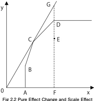
As Figure 2.2 shows, 0CG is the production frontier with constant returns to scale. BCD is the production frontier with non-constant returns to scale. Suppose E is an arbitrary point in the production possibility set, the efficiency change will be expressed by FE/FG with constant returns to scale. However, if the technology is not neutral, the efficiency change should be sepa-rated into two parts, pure effect change and scale effect. In the above figure they are expressed by FE/FD and DG. The scale effect is therefore defined as the ratio of the two efficiency chang-es(Forsund and Hjalmarsson,1979).
To summarize, the Malmquist index can be used to compare the efficiency change and tech-nological progress in different time periods. Considering the scale effect, the Malmquist index can be decomposed as
y
0
A
B
C
D
E
G
F
x
Fig 2.2 Pure Effect Change and Scale Effect
where Effch stands for efficiency change, and represents how close the given observations approach the production frontier. This index being greater than 1 indicates an increase in efficiency. Techch represents technological change; this number being larger than 1 indicates technological progress in given observations. Effch can be further expressed by the product of Pech and Sech, which stands for pure efficiency change and scale effect respectively.
2.2 Data source and variable definition
The provincial TFP calculation is based on provincial GDP, labor and capital stock. In this paper we use data from years 1978 to 2007. Provincial real GDP are deflated with 1978 as the base year. The data of earlier years come from Comprehensive Statistical Data and Materials on 50 Years of New China 1949-1999 (NBS of China, 1999). The data of later years (1995-2007)
come from China’s statistical year books. Note that a large portion of data in Tibet and Hainan
province were missing, therefore we omitted these two provinces from our observations. Since Chongqing was part of Sichuan province and did not become an independent province until 1997, for consistency we combine the data of Sichuan and Chongqing after 1997 into one obser-vation. The total number of observations is 28.
The calculation of stock capital follows a perpetual inventory method with 1978 as the base year. For example the capital stock in 1979 equals the amount of fixed investment in this year multiplied by investment price index, then plus depreciated capital stock from 1978. Here we take depreciation ratio to be 9.6% (Jun Zhang, 2006). Labor stock in this paper is represented by the number of employees (Jinxu Cai, 2000; Yumin Ye, 2002).
2.3 Trend of China’s TFP
According to the fluctuation, trend and composition of TFP, we divide the evolution of
Chi-na’s TFP from 1979 to 2007 into the following periods.
From 1979 to 1991, the TFP fluctuated largely with an increasing absolute value. This is mainly caused by efficiency change (average = 2%). The technological progress was negative in 1978 since at that time China was in the transaction from planned economy to market economy, and the allocation of resources can not meet the need of the new institution. Since 1989, tech-nological progress becomes the major contributing factor instead of efficiency change. As we can see from Figure 2.3, the technological progress curve is above the efficiency change curve from 1989. Two factors lead to this change. First, during the late 1980s the Chinese government adopted a series of policies promoting the commercial application of technological innovations. Second, the price reform in 1988 resulted in small fluctuations in economic growth. The TFP thus exhibited a small decrease, followed by rapid rise with constant 4% increase rate.
From 1992 to 1996, we observe a decreasing TFP, which is largely affected by slower
tech-nological progress. One reason may be that China’s investment in scientific and technological
research declined during this time period; it may also result from a slow adoption of foreign
technology. For example, the growth of China’s Three Types of Expenditure in Science and
Technology reduced from 30% in 1990 to 13.13% in 1992. From 1994 to 1995, the growth of the Three Types of Expenditure became negative (-14.92%). From 1993 to 1996, the growth of for-eign investment also slowed down: the growth was 152.46% during 1990 to 1992, while it was only 16.95% from 1993 to 1996. Meanwhile, at this time period China experienced overcapacity and inflation. The domestic market transited from shortage to surplus.
During 1997 to 2004, the TFP stabilized with slowed down technological progress decline. The most evident characteristic of this period is the significant impact of technological progress on TFP growth. This indicates that with the institutional reform, the allocation of resources began to adapt to the market demands. The technological progress through innovation and imitating foreign technology began to have a larger impact in TFP than efficiency change. Scale benefit was far smaller than that in 1980s. The decreasing efficiency change also indicates a larger gap between actual output level and the production frontier.
During 2005 to 2007, The TFP displayed slight fluctuations. Both decline in technologi-cal progress and efficiency change are observed. Further investigation is needed to conclude whether such trend will retain.
2.4 Comparative study of provincial TFP
The data pool includes GDP, labor force and capital stock of 28 provinces in the past 30 years. We will use our analysis results of provincial TFP and its components to compare over time and across regions.
Table 2.2 lists the provincial TFP and its decomposition. The average provincial TFP during 1978-2007 is 1.022, which shows in this time period the regional economies progressed in scale ef-ficiency, efficiency of productive factor usage, and technological progress. The TFP growth was
largely driven by technological progress, which is inconsistent with Wu’s (2002) findings that it
Table2.1 China’s TFP change and its components (1979 - 2007)
Year Efficicency Change Technological progress Pure Efficiency Change Scale Effect TFP Change
1979 1.0180 1.0040 1.0240 0.9940 1.0220 1980 1.0210 1.0090 1.0200 1.0010 1.0300 1981 1.0390 0.9710 1.0200 1.0190 1.0080 1982 1.0740 0.9680 1.0550 1.0190 1.0400 1983 1.0670 0.9750 1.0490 1.0180 1.0410 1984 1.0690 1.0020 1.0310 1.0370 1.0710 1985 1.0240 1.0090 0.9980 1.0260 1.0330 1986 1.0410 0.9450 1.0240 1.0160 0.9840 1987 1.0460 0.9700 1.0320 1.0130 1.0140 1988 1.0250 1.0020 1.0040 1.0210 1.0270 1989 0.9930 0.9930 0.9960 0.9980 0.9860 1990 0.9780 1.0180 0.9860 0.9910 0.9960 1991 0.9580 1.0670 0.9760 0.9820 1.0230 1992 0.9670 1.0990 0.9680 0.9990 1.0620 1993 0.9720 1.0800 0.9700 1.0020 1.0500 1994 0.9780 1.0550 0.9790 0.9990 1.0330 1995 1.0030 1.0230 1.0000 1.0040 1.0260 1996 1.0200 1.0070 1.0050 1.0150 1.0270 1997 1.0020 1.0220 1.0080 0.9940 1.0240 1998 1.0120 1.0020 1.0100 1.0020 1.0140 1999 0.9990 1.0160 0.9960 1.0030 1.0150 2000 0.9990 1.0120 1.0010 0.9980 1.0110 2001 0.9920 1.0170 1.0000 0.9920 1.0090 2002 0.9850 1.0260 0.9890 0.9950 1.0100 2003 0.9820 1.0300 0.9890 0.9930 1.0120 2004 0.9790 1.0320 0.9970 0.9820 1.0110 2005 1.0100 1.0100 1.0100 1.0000 1.0200 2006 1.0400 1.0590 1.0150 1.0250 1.1020 2007 1.0200 1.0030 0.9740 0.9680 1.0170
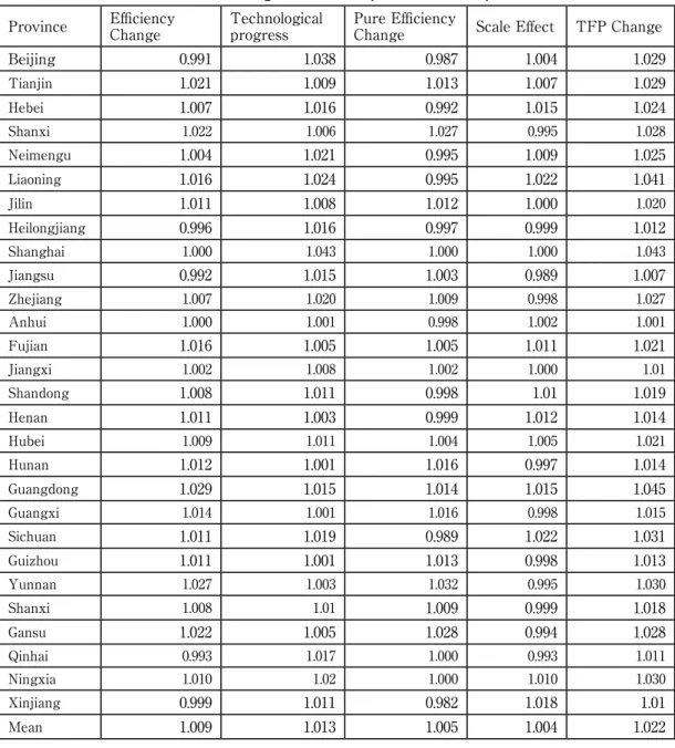
Among all the provinces, Shanghai and Guangdong have the highest TFP (4.3% and 4.5% respectively). However, the sources of TFP increase in these two provinces are different.
Shang-hai’s TFP is largely influenced by technological progress while Guangdong’s TFP was mainly
affected by efficiency change. In Shanghai, the effects of industrial clusters as well as increasing FDI and skilled workers promoted the technological progress. In Guangdong technology and efficiency was improved through imitation and learning
0.8500 0.9000 0.9500 1.0000 1.0500 1.1000 1.1500 1979 1980 1981 1982 1983 1984 1985 1986 1987 1988 1989 1990 1991 1992 1993 1994 1995 1996 1997 1998 1999 2000 2001 2002 2003 2004 2005 2006 2007
year
efficiency change
technical progress
TFP
Fig2.3 TFP and its components over time
In the paper we also calculated the TFP and its components of eastern China, central Chi-na and western ChiChi-na. As shown in figure 2.4, before 1990 all three regions share similar rate of TFP. The eastern region has the fastest TFP growth afterwards. The main reason for this phenomenon is that during the earlier years of economic reform, the differences of technology and policies was not yet obvious across regions, while later on the eastern region became more open and attracted more economic resources. Therefore this region displayed a most significant improvement in technology and production efficiency.
With regard to the efficiency change, the efficiency change indexes were increasing in all regions from 1981 to 1985 (Figure 2.5). The average efficiency change was approximately 6%. The western region
enjoyed a larger catch-up growth and it’s been approaching the eastern region since 1990. Before 1990,
efficiency change was mainly attributed to effect of institution. Since the institution reform and economic policies were universal and indifferent across China, there were no significant differences in efficiency among regions. From 1990, the eastern region is more open and attracts more economic resources and technology. As a result it has a higher efficiency index curve which surpasses the western and the cen-tral until 1995. Later on, the efficiency growth of the latter two regions accelerated with a faster speed that overtook the eastern region. As discussed before, the efficiency change can be divided into pure efficiency change and scale effect. The western and central regions benefited from the scale effect by expanding its production capacity; the eastern region, on the other hand, faced a decreasing scale effect.
Concerning the technological progress, all three regions displayed a similar pattern. From figure 2.6 we see that during 1979 to 1993, the three technological progress curves converge with average growth equals 3% to 4%. In the early years of the economic reform, the difference in regional
develop-ment mainly resulted from scale economy effect rather than technological progress. In 1994, China’s
reform involved in various areas including finance, foreign trade, state owned enterprises, social securi-ty, etc. The power and influence of such reform in the eastern region is different from that in the west and the central. Meanwhile, the optimization of industrial structure, adoption of advanced technology, and the update of products were faster in the eastern region than the west and the central.
Table 2.2 TFP change and its components across provinces
Province Efficiency Change Technological progress Pure Efficiency Change Scale Effect TFP Change
Beijing 0.991 1.038 0.987 1.004 1.029 Tianjin 1.021 1.009 1.013 1.007 1.029 Hebei 1.007 1.016 0.992 1.015 1.024 Shanxi 1.022 1.006 1.027 0.995 1.028 Neimengu 1.004 1.021 0.995 1.009 1.025 Liaoning 1.016 1.024 0.995 1.022 1.041 Jilin 1.011 1.008 1.012 1.000 1.020 Heilongjiang 0.996 1.016 0.997 0.999 1.012 Shanghai 1.000 1.043 1.000 1.000 1.043 Jiangsu 0.992 1.015 1.003 0.989 1.007 Zhejiang 1.007 1.020 1.009 0.998 1.027 Anhui 1.000 1.001 0.998 1.002 1.001 Fujian 1.016 1.005 1.005 1.011 1.021 Jiangxi 1.002 1.008 1.002 1.000 1.01 Shandong 1.008 1.011 0.998 1.01 1.019 Henan 1.011 1.003 0.999 1.012 1.014 Hubei 1.009 1.011 1.004 1.005 1.021 Hunan 1.012 1.001 1.016 0.997 1.014 Guangdong 1.029 1.015 1.014 1.015 1.045 Guangxi 1.014 1.001 1.016 0.998 1.015 Sichuan 1.011 1.019 0.989 1.022 1.031 Guizhou 1.011 1.001 1.013 0.998 1.013 Yunnan 1.027 1.003 1.032 0.995 1.030 Shanxi 1.008 1.01 1.009 0.999 1.018 Gansu 1.022 1.005 1.028 0.994 1.028 Qinhai 0.993 1.017 1.000 0.993 1.011 Ningxia 1.010 1.02 1.000 1.010 1.030 Xinjiang 0.999 1.011 0.982 1.018 1.01 Mean 1.009 1.013 1.005 1.004 1.022
3. AN ANALYSIS ON THE INFLUENCING FACTORS OF PROVINCIAL TFP
3.1 Influencing factors of efficiency change and technological progress
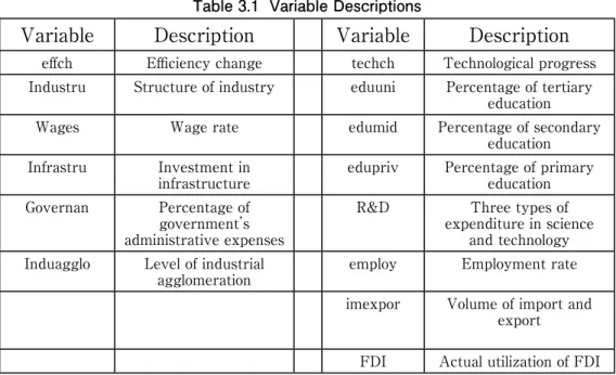
There are many factors that would influence technological progress. However, in the case of China, the main factors are investment in science and technology, spillover effect of foreign technology, stock of human capital and the investment in education. In this paper we choose 7 variables to represent the above aspects: percentages of people who receive primary, secondary and tertiary education as their highest level of education, three types of expenditure in science and technology, employment rate, total import and export volume, and the actual utilization of foreign investment (Table 3.1).
Fig2.4 Regional Comparison on TFP
Fig2.5 Regional comparison on efficiency change
There are also numerous influencing factors for the improvement of a country’s efficiency. In this
paper the variables we are interested in are industrial structure, wage rate, investment in infrastructure,
percentage of government’s administrative expenses and the level of industrial agglomeration (Table 3.1).
Variable definition:
Level of industrial agglomeration = gross output of secondary sector in the given province / gross output of secondary sector in the whole country;
Fig2.6 Regional comparison on technological progress
Actual utilization of FDI = foreign investment utilized / total foreign investment;
Volume of import and export: converted into RMB using annual average exchange rates; Employment rate = number of employed people / total population;
Education: primary education = 6 years, secondary = 9 years, tertiary education = 16 years; data come from survey of population above the age of 6;
Wage rate = average wage rate of employed population in given province;
Investment in infrastructure = the amount of expenses in infrastructure out of total fiscal ex-penditure;
Three types of expenditure in science and technology: government project funds supporting the trial manufacture of new products, intermediate experiments and major scientific projects. These expenses account for a large portion in total R&D expenditure;
Percentage of government administrative expenses = government administrative expenses / GDP; this ratio can be used as an indicator of the transaction cost of promoting production; Structure of industry = growth of second and third sectors / growth of the first sector.
3.2 Data source
Most provincial data come from China Statistical Yearbook, Comprehensive Statistical Data and Materials on 50 Years of New China 1949-1999 and Data of Gross Domestic Product of China 1952-2004 with exceptions otherwise noted. We choose data from 1990 to 2007 for the following reasons. First, during the period of 1978 to 1990, a large portion of data is missing.
Second, from the previous analysis we know that China’s total factor productivity dropped for
the first time in early 1990s. Therefore we should regard this turning point as a crucial part of our analysis. Third, in the early 1990s China was experiencing an acceleration of transition to market economy. Using 1990 as the starting point will enable us to capture the change of the above variables during this time period.
Table 3.1 Variable Descriptions
Variable
Description
Variable
Description
effch Efficiency change techch Technological progress
Industru Structure of industry eduuni Percentage of tertiary education
Wages Wage rate edumid Percentage of secondary
education Infrastru Investment in
infrastructure edupriv Percentage of primary education Governan Percentage of
government’s administrative expenses
R&D Three types of expenditure in science
and technology Induagglo Level of industrial
agglomeration employ Employment rate
imexpor Volume of import and export
FDI Actual utilization of FDI
3.3 Model of influencing factors of TFP and its applications
As mentioned above, in this paper we study 5 variables that affect the efficiency change and 7 variables that affect the technology progress. On this basis we establish the following model:
(3-1) (3-2)
For province i at time t, the x’s are industru, wages, infrastru, governan and induagglo and
the y’s are eduuni,edumid,edupriv,R&D,employ,imexpor and FDI.
3.3.1 Model testing
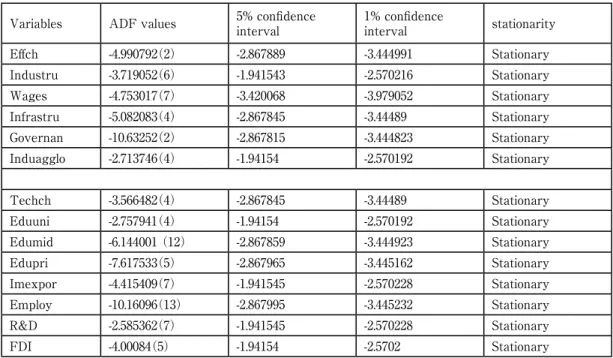
(1) ADF unit root testing
In order to avoid spurious regression problems, this paper uses ADF unit root testing meth-od for the stationary test of the dependent and independent variables.
From table 3.2 we see that after adjustment for time lags (number of lags are indicated in the parentheses), the absolute values of the ADF test results for all variables are greater than the absolute values of the 1% confidence interval, which means all the variables are stationary. We selected the optimal number of lags by minimizing the AIC and Schwarz number, i.e., the
parameter p that minimizes the AIC and SC values is taken as the optimal number of lags. Taking the variable “Wages” as an example:
Table 3.2 ADF Unit Root Test
Variables ADF values 5% confidence interval 1% confidence interval stationarity
Effch -4.990792(2) -2.867889 -3.444991 Stationary Industru -3.719052(6) -1.941543 -2.570216 Stationary Wages -4.753017(7) -3.420068 -3.979052 Stationary Infrastru -5.082083(4) -2.867845 -3.44489 Stationary Governan -10.63252(2) -2.867815 -3.444823 Stationary Induagglo -2.713746(4) -1.94154 -2.570192 Stationary Techch -3.566482(4) -2.867845 -3.44489 Stationary Eduuni -2.757941(4) -1.94154 -2.570192 Stationary Edumid -6.144001 (12) -2.867859 -3.444923 Stationary Edupri -7.617533(5) -2.867965 -3.445162 Stationary Imexpor -4.415409(7) -1.941545 -2.570228 Stationary Employ -10.16096(13) -2.867995 -3.445232 Stationary R&D -2.585362(7) -1.941545 -2.570228 Stationary FDI -4.00084(5) -1.94154 -2.5702 Stationary
Table 3.3 Choice of lags for “Wages”
Lag Akaike info criterion Schwarz criterion
1 18.87242 18.90920 2 18.86760 18.91365 3 18.86904 18.92439 4 18.85546 18.92014 5 18.86067 18.93472 6 18.84846 18.93191 7 18.70236 18.79524 8 18.70855 18.81089
From the table 3.3 we can see the AIC and Schwarz values are minimized when number of lags equals seven. Therefore we choose seven as the optimal number.
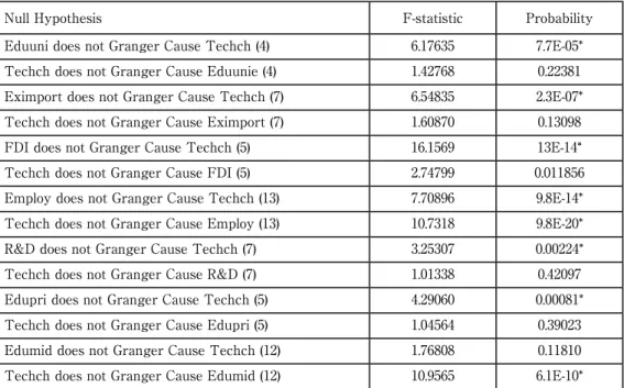
Table 3.4 Granger Causality Test on Technological progress
Null Hypothesis F-statistic Probability
Eduuni does not Granger Cause Techch (4) 6.17635 7.7E-05* Techch does not Granger Cause Eduunie (4) 1.42768 0.22381 Eximport does not Granger Cause Techch (7) 6.54835 2.3E-07* Techch does not Granger Cause Eximport (7) 1.60870 0.13098 FDI does not Granger Cause Techch (5) 16.1569 13E-14* Techch does not Granger Cause FDI (5) 2.74799 0.011856 Employ does not Granger Cause Techch (13) 7.70896 9.8E-14* Techch does not Granger Cause Employ (13) 10.7318 9.8E-20* R&D does not Granger Cause Techch (7) 3.25307 0.00224* Techch does not Granger Cause R&D (7) 1.01338 0.42097 Edupri does not Granger Cause Techch (5) 4.29060 0.00081* Techch does not Granger Cause Edupri (5) 1.04564 0.39023 Edumid does not Granger Cause Techch (12) 1.76808 0.11810 Techch does not Granger Cause Edumid (12) 10.9565 6.1E-10*
(2) Granger causality test
Since the variables are stationary, we can use granger causality test to test for the causal relationship between total factor productivity and the variables.
We use the same method above to determine the number of lags. Table 3.4 shows that under 1% significance level there is a causal relationship between technological progress and 6 vari-ables: percentage of population with tertiary education, percentage of population with primary education, total import and export, foreign direct investment, employment rate and R&D. Among these variables, the employment rate and technological progress interlinked with each another, indicating that the employment rate can stimulate the technological progress while vice versa.
Using similar method we run the same causality test on efficiency change and relevant variables:
3.3.2 Economic meaning of the model
In this paper we use a fixed effects model to analyze our panel data, and the results are as follow.
3.3.2.1 Analysis of technological progress
In the fixed effects model with the technological progress as the dependent variable, the R-squared reaches 0.990608, indicating a high fitness of the model. The DW test statistic indi-cates that we can not rule out the possibilities of residual autocorrelation. However, since the cross section of the panel data is often large, often we only have the time demeaned error esti-mates, and the DW statistic is unlikely the error in the original model.
Table 3.5 Granger Causality Test on Efficiency Change
Null Hypothesis F-statistic Probability
Industru does not Granger Cause effch (6) 3.64921 0.01271 Effch does not Granger Cause Industru (6) 0.23939 0.86887 Wages does not Granger Cause Effch (7) 1.42655 0.16578 Effch does not Granger Cause Wages (7) 0.76552 0.66218 Infrastru does not Granger Cause Effch (4) 5.38137 0.00941* Effch does not Granger Cause Infrastru (4) 2.74799 0.99563 Governan does not Granger Cause Effch (13) 2.21178 0.00214* Effch does not Granger Cause Governan (13) 0.55205 0.94257* Induagglo does not Granger Cause Effch (4) 2.21725 0.00208* Effch does not Granger Cause Induagglo (4) 2.44197 0.00058*
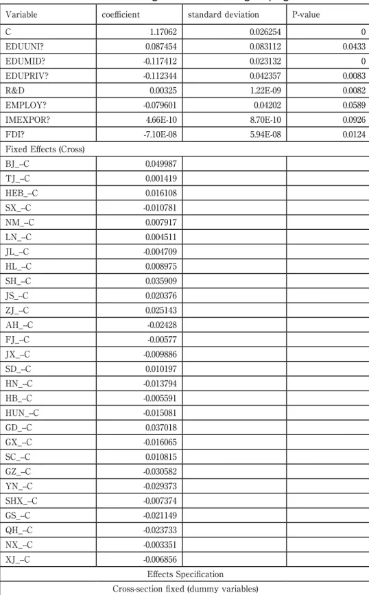
(1) Education and technological progress.
Our results show a negative relationship between the technological progress and the per-centage of population with primary (coefficient -0.1123) and secondary (coefficient -0.1174)
edu-cation as their highest level of eduedu-cation, which is opposite to Phelps’s views. However in the
case of China, since the implementation of compulsory education, the attendance rate of primary school has reached 99.54% in 2008, which means primary and even secondary education has been carried out universally. Therefore a further widespread of primary and secondary educa-tion is not enough to motivate technological innovaeduca-tion; it is the level of tertiary educaeduca-tion that most promotes technological progress. From the results above we indeed see a positive relation between tertiary education and technological progress.
(2) Investment in R&D and technological progress.
It can be intuitive that investment in R&D has a positive relation with technological prog-ress. The former directly motivates new products and technology. In our model the estimated coefficient for R&D is 0.00325, a positive but rather small number. This may be explained by the fact that we only use the three types of expenses in science and technology as an indicator of R&D investment, and we have not include information on the investment in R&D from pri-vate companies or organizations. However we cannot exclude the possibility that the influence of R&D investment in indeed low in China; for example there may be inefficiency in the actual usage of the government funds.
(3) Employment rate and technological progress.
The influence of employment rate on technology progress is negative but insignificant. Since Chinese industries are still labor intensive, employment rate does not have a significant relation-ship with technological progress.
Table 3.6 Influencing factors of technological progress Variable coefficient standard deviation P-value
C 1.17062 0.026254 0 EDUUNI? 0.087454 0.083112 0.0433 EDUMID? -0.117412 0.023132 0 EDUPRIV? -0.112344 0.042357 0.0083 R&D 0.00325 1.22E-09 0.0082 EMPLOY? -0.079601 0.04202 0.0589
IMEXPOR? 4.66E-10 8.70E-10 0.0926
FDI? -7.10E-08 5.94E-08 0.0124
Fixed Effects (Cross)
BJ_--C 0.049987 TJ_--C 0.001419 HEB_--C 0.016108 SX_--C -0.010781 NM_--C 0.007917 LN_--C 0.004511 JL_--C -0.004709 HL_--C 0.008975 SH_--C 0.035909 JS_--C 0.020376 ZJ_--C 0.025143 AH_--C -0.02428 FJ_--C -0.00577 JX_--C -0.009886 SD_--C 0.010197 HN_--C -0.013794 HB_--C -0.005591 HUN_--C -0.015081 GD_--C 0.037018 GX_--C -0.016065 SC_--C 0.010815 GZ_--C -0.030582 YN_--C -0.029373 SHX_--C -0.007374 GS_--C -0.021149 QH_--C -0.023733 NX_--C -0.003351 XJ_--C -0.006856 Effects Specification Cross-section fixed (dummy variables)
Weighted Statistics
R-squared 0.990608 Mean dependent var 1.171319
Adjusted R-squared 0.989835 S.D. dependent var 0.324661 S.E. of regression 0.032732 Sum squared resid 0.442492
F-statistic 1281.257 Durbin-Watson stat 0.867092
Prob(F-statistic) 0
Unweighted Statistics
R-squared 0.262092 Mean dependent var 1.032525
Sum squared resid 0.445094 Durbin-Watson stat 0.855645
(4) Import-export volume and technological progress.
Import-export volume has a significant positive relationship with technological progress. This indicates that foreign technology spillover and the imitation of foreign technology has
positively influenced China’s technological progress. The competition in the global market
push-es the production frontier forward and optimized the scale of Chinpush-ese enterprispush-es. However, though being positive, the coefficient is quite small (4.66E-10). From the perspective of import, though the import of hi-tech products has created the chance of imitating foreign technology, most of the imports are the semi-finished materials to be used on the exported goods (Bing Hu and Jing, Qiao, 2008) which do not have much potential for the learning of technology. From the perspective of export, although the quality and structure of the exported goods have been
greatly improved during recent years, China’s exported good still cannot compete with other
countries in terms of quality and added-value and it doesn’t play an important part in
stimulat-ing the progress of technology (Yuan Shu, 1998). Therefore we can conclude that the influence of import and export volume on technological progress is still limited.
(5) Actual utilization of FDI and the technological progress.
FDI has a small negative influence on technological progress according to our results. FDI not only brings funds but also brings advanced technology and management methods. As Changyuan Luo (2006) found out, FDI creates better conditions for the growth of TFP. In gen-eral, there is a time lag between the introduction of foreign technology and its full absorption which is partly dependent on local features such as local technology and human resource. If the local features are unfavorable, the cost of learning and absorbing time will correspondingly increase.
(6) Provincial features.
Beijing, Shanghai and Guangdong have the largest constant term among the 28 provinces; the constant term for western provinces such as Guizhou and Gansu are relatively smaller. This indicates a relationship between regional features and technological progress. Eastern provinc-es have advantagprovinc-es in infrastructure, policiprovinc-es and human capital stock which lead to a larger technological progress. Western provinces are still restricted by regional features though they have a fast catch-up growth.
3.3.2.2 Analysis of efficiency change
Table 3.7 Influencing factors of Efficiency Change Variable Coefficient Standard Deviation P-value
INDUSTRU? 0.000246 0.000171 0.0028
WAGES? 6.18E-07 3.01E-07 0.0409
INFRASTRU? 4.72E-10 4.48E-09 0.0162
GOVERNAN? -0.171612 0.042883 0.0001
INDUAGGLO? 0.130705 0.164362 0.4269
Fixed Effects (Cross)
BJ_--C 0.005104 TJ_--C 0.030667 HEB_--C -0.004132 SX_--C 0.010497 NM_--C -0.020794 LN_--C 0.030333 JL_--C -0.004317 HL_--C -0.005044 SH_--C 0.031501 JS_--C -0.00777 ZJ_--C -0.011553 AH_--C -0.020037 FJ_--C -0.000594 JX_--C -0.014848 SD_--C 0.008947 HN_--C -0.00342 HB_--C -0.014656 HUN_--C 0.00234 GD_--C 0.021231 GX_--C -3.28E-05 SC_--C 0.020719 GZ_--C -0.012576 YN_--C 0.009219 SHX_--C -0.009209 GS_--C 0.003012 QH_--C -0.021502 NX_--C -0.002714 XJ_--C -0.020372 Effects Specification Cross-section fixed (dummy variables)
R-squared 0.999391 Mean dependent var 2.102665 Adjusted R-squared 0.999344 S.D. dependent var 1.685321 S.E. of regression 0.043153 Sum squared resid 0.772809
F-statistic 21292.87 Durbin-Watson stat 1.134434
Prob(F-statistic) 0
Unweighted Statistics
R-squared 0.082396 Mean dependent var 0.990507
Sum squared resid 0.869232 Durbin-Watson stat 1.154326
We estimate a fixed effects model of the efficiency change, and the results are shown in table 3.7. The R-squared for our model is 0.999391, indicating a high fitness of the model.
(1) Industry structure and efficiency change.
The industry structure is measured by the ratio of added-value in second and third sectors to the added-value in the first sector. It has a positive influence on efficiency change (0.000246).
(2) Wage rate and efficiency change.
The influence of wage rate on efficiency change is not significant as it has not passed the 5% significance level.
(3) Investment in infrastructure and efficiency change.
Investment in infrastructure has a positive relationship with efficiency change. To some extent it gives the less developed provinces an opportunity to catch up with the developed provinces through investment in infrastructure. According to the study of Dina Jiang (2003), the TFP of railway transportation industry is rising with significant scale effect. Driven by fixed investment after the 90s, the development of road transportation improves the efficiency of less developed area, especially the western region. Affected by the growth of fixed investment, civil aviation industry has scale effect, and its development boosts the economic efficiency of developed provinces.
(4) Government administrative expenses and efficiency change.
Government’s administrative expenses have a significant negative effect on efficiency change.
On the one hand, the intervention of government may reduce the efficiency of capital and labor input; on the other hand, higher administrative expenses in proportion to other expenses also indicate that the cost of governance has a low efficiency in driving the economy.
(5) Industrial agglomeration and efficiency change.
Industrial agglomeration can reduce the transaction costs among enterprises and improve efficiency through positive externalities. In accordance with this theory, our model displayed a positive relationship between industrial agglomeration and efficiency change.
4. CONCLUSION
periods: From 1979 to 1991, following a rapid growth in Chinese economy, the TFP increased from negative to positive. From 1992 to 1996, while the speed of economic growth was still high, the growth of the TFP began to slow down. From 1997 to 2004, with high economic growth, the growth of TFP tended to be stable, despite a decline in technological progress. During 2005 to 2007 there was a small fluctuation in the TFP; both technological progress and efficiency change started to decline after a small peak. However since we do not have further data, the observa-tions in these three years are not enough for us to draw any conclusion on future TFP trend.
The analysis in this paper also reveals different TFP levels among the eastern re-gion, western region and the central region. Such difference was not obvious from 1979 to 1989;
however the gap enlarged from 1990 to 2007. This can be explained by the fact that China’s
economic reform has a larger impact in the eastern region; fast industrial development, increas-ing foreign trade and foreign investment enabled the firms in the eastern region to obtain new technology and learn new techniques, which in turn resulted in a larger technological progress compared with the west and the central.
In the paper we also studied the influencing factors for technological progress and effi-ciency change. Among the relevant variables, the proportion of population with tertiary educa-tion, R&D investment and the actual utilization of FDI have significant effect on the progress of technology; the industrial structure and government administration expenses have a significant influence on efficiency change. The difference in the constant terms of the model indicates that provincial features, such as infrastructure, government policies and human resource, also affect technological progress or efficiency change.
References
1 World Bank. China 2020: Development Challenges in the New Century. Washington D.C.: The World Bank, 1997.
2 National Bureau of Statistics of China. China Statistical Yearbook. 1999-2008, China Statis-tics Press.
3 National Bureau of Statistics of China. Comprehensive Statistical Data and Materials on 50 Years of New China 1949-1999. China Statistics Press, 1999.
4 HU, Angang. China’s future development depends on TFP.
http://www.china.com.cn/authority/txt/2002-07/04/content_5168635.htm, July 4 2002.
5 SACHS, Jeffrey D. and WOO, Wing Thye. Understanding China’s Economic Performance.
NBER Working Paper No. W5935. 1997.
6 BHATTASALI, Deepak. Sustaining China’s Development: Some Issues. Presentation to
Tsinghua University 90th Anniversary Celebrations Seminar Series, Beijing, People’s
Re-public of China, April 24, 2001.
Companies and its determinants in 1990-1994. Economic Research Journal. 1999(7).
8 ZHANG, Jun. China’s industrial reform and economic growth: problems and explanation.
Shanghai: Shanghai Renmin Press, 2003.
9 WANG, Yan and YAO, Yudong. Sources of China’s economic growth 1952-1999:
incorporat-ing human capital accumulation. China Economic Review, 2003, 14(1): 32–52.
10 ZHEN Jinhai and HU Angang. A positive analysis on changes of provincial productivity
growth during China’s reform. Chinese Economic Quarterly, 2005(1): 263-296.
11 LI, Shengwen, and LI, Dasheng. Regional differences of TFP in China. The Journal of Quan-titative & Technical Economics, 2006(9): 12-21.
12 SHEN, Neng. An empirical analysis on total factor productivity diversity in china’s
manu-facturing industry. China Soft Science, 2006(6).
13 LI, Jinwen and GONG, Feihong. Productivity and China’s economic growth. The Journal of
Quantitative & Technical Economics,1996(12): 27-40
14 CHAMARBAGWALA, Ubiana, RAMASWAMY, Sunder and WUNNAVA, Hanindra V. The Role of Foreign Capital in Domestic Manufacturing Productivity: Empirical Evidence from Asian Economies. Applied Economies. 2000(32): 393-398.
15 WANG, Xiaolu. Sustainability and regulational change of China’s economic growth.
Eco-nomic Research Journal, 2000(7): 53-54.
16 KUMAR, S. and RUSSELL, R. Technological Change, Technological Catch-Up, and Capital Deepening: Relative contributions to Growth and Convergence. American Economic Re-view, 2002, 92(3): 527-548.
17 GUO, Qinwang and JIA, Junxue. Estimates of total factor productivity in China: 1979-2004. Economic Research Journal, 2005(6): 51-60.
18 WANG, Zhigang, GONG, Liutang and CHEN, Yuyu. Inter-regional productivity and decom-postion of TFP (1978-2003). Social Sciences in China, 2006, 158(3): 45-54.
19 SHI, Qingqi. An analysis on measures to accelerate technological advances. Development Research, 1986.
20 JEFFERSON, Gary, THOMAS, Rawski, WANG, Li and ZHENG, Yuxin. Ownership, Produc-tivity Change and Financial Performance in Chinese Industry, Journal of Comparative Economics, 2000, 28(4): 786-813.
21 TIMMER, Marcel P. and SZIRMAI, Adam. Productivity Growth in Asian Manufacturing: The Structural Bonus Hypothesis Examined. Applied Economics, 2000(30): 121-132.
22 ROMER, Paul M. Capital, labor and productivity. Brookings Papers on Economic Activity. Microeconomics, 1990: 337-367.
23 BENHABIB, Jess and SPIEGEL, Mark M. The Role of Human Capital in Economic Devel-opment:Evidence from Aggregate Cross-Country Data. Journal of Monetary Economics,
1994, 34(2): 143-73.
24 BERNSTEIN, Jeffrey I. and YAN, Xiaoyi. International R&D Spillovers between Canadian and Japanese Industries. Canadian Journal of Economics, 1997, 30(2): 276-94.
25 MADDEN, Gary, SAVAGE, Scott J, and BLOXHAM, Paul. Asian and OECD international R&D spillovers. Applied Economics Letters, 2001, 8(7): 431-435.
26 ATELLA, Vincenzo and QUINTIERI, Beniamino. Do R&D Expenditures Really Matter for TFP? Applied Economics, 2001, 33(11): 1385-1389.
27 EGAN, Mary Lou and MODY, Ashoka. Buyer-seller links in export development. World Development, 1992, 20(3): 321-334.
28 COE, David T., HELPMAN, Elhanan, and HOFFMAISETER, Alexander W. North-South R & D Spillovers. The Economic Journal, 1997, 107: 134-149.
29 GEREFFI, G.ary. A commodity chains framework for analyzing global industries. Institute of Development Studies, 1999.
30 WEI, Mei. Regional TFP factors and analyses on convergence of efficiencies. Statistics and Decision, 2008(12): 77-79.
31 LIU, Binglian and LIU, Yong. Regional characters’ impact on TFP in Hebei province.
Jour-nal of Heibei University (Arts & Social Science Section), 2006(3): 19-24.
32 WANG, Yingwei and CHENG, Bangwen. A quantitative analysis regarding the effects of
China’s research and development on TFP. Science and Technology Management
Re-search, 2005, 25(6): 39-42.
33 YUAN, Peng, CHEN, Xin and HU, Rong. An empirical research on the effect of internation-al trade to technicinternation-al efficiency. Forecasting, 2005(6): 52-55.
34 HUANG, Yanlin. An analysis on several factors affecting China’s technological progress.
Market Modernization, 2006(35):370-371.
35 CHEN, Jianbao and DAI, Pingsheng. Impact of Fiscal Expenditure on Economic Growth in China: an analysis of its multiplier effect. Journal of Xiamen University (Arts & Social Sci-ences), 2008(5):26-32.
36 YUE, Shujin and LIU, Chaoyang. An analysis on human capital and regional TFP. Journal of Economic Research, 2006:90-96.
37 FORSUND, Finn R. and HJALMARSSON, Lennart. Frontier production functions and tech-nological progress: a study of general milk processing in Swedish Dairy Plants. Economet-rica. 1979, 47(4): 883-900.
38 NELSON, Richard R. and PHELPS, Edmund S. Investment in humans, technological diffu-sion, and economic growth. American Economic Review, 1966, 56(2): 67-75.
39 ROSTOW, W. W. The stages of economic growth: A Non-Communist Manifesto,Cambridge:
40 KNUDSEN, D. Shift-share analysis: Further examination of models for the description of economic change. Socio-Economic Planning Sciences, 2000, 34: 177-198.
41 CANNING, David, MARIANNE, Fay and ROBERTO, Perotti. Infrastructure and Growth, in Mario Baldassarri, Luigi Paganetto, Edmund Phelps(eds). International differences in Growth rates. New York: Mavmillan Press, 1994: 113-417.
42 ASCHAUER, David Alan. Is public expenditure productive? Journal of Monetary Econom-ics, 1989(2): 177-200.
43 CHATTERJEE, Santanu, SAKOULIS, Georgios and TURNOVSKY, Stephen. Unilateral capital transfers, public investment, and economic growth. European Economic Reviews, 2003, 47(6):1077-l103.
44 HU, Angang and ZHEN Jinhai. Why does China’s TFP significantly decrease? China
Eco-nomic Times, 2004(3).
45 ZHEN, Jinhai and HU, Angang. Empirical analysis on the changes of inter-provincial TFP
during China’s reform. Quarterly Journal of Economics, 2005(1):263-296.
46 Website of Ministry of Finance of P. R. China: http://www.mof.gov.cn/index.htm
47 JIANG, Dianchun and ZHANG, Yu. Industrial characteristics and spillover of foreign direct investment: an empirical analysis based on high-tech industry. The Journal of World Econ-omy. 2006(10): 21-29.
48 LIU, Wei and ZHANG, Hui. Changes in industrial structure and technological progress
during China’s economic growth. Journal of Economic Research, 2008(11).
49 ZHU, Jiejin and HU, Yongping. Governmental expenditure, productivity improvement and economic growth: an empirical study based on panel data and random coefficient model. Contemporary Finance & Economics, 2005(2):15-18.
50 CHOW, Gregory. Capital Formation and Economic Growth in China. The Quarterly Journal of Economics, 1993, August.