特異値計算のmdLVsアルゴリズムと特異値分解のI-SVDアルゴリズムにおける最近の進展 (流体計算における高速アルゴリズムの理論とその応用)

Recent Developments

of

the

mdLVs Algorithm

for

_{Singular Values}

and the

I-SVD

Algorithm

for Singular

Value

Decomposition

特異値計算の

mdLVs

アルゴリズムと

特異値分解の

I-SVD

アルゴリズムにおける最近の進展

京都大学情報学研究科 中村佳正1(Yoshimasa Nakamura)

Graduate SchoolofInformatics, Kyoto University

京都府立大学人間環境学部 岩崎雅史 (Masashi Iwasaki)

Faculty ofHuman Environment, KyotoPrefectural University

京都大学情報学研究科 木村欣司 (KinjiKimura)

Graduate School ofInformatics, Kyoto University

奈良女子大学人間文化研究科 高田雅美 (Masami Takata)

Graduate School of Humanitics

&

Sciences, NaraWomen’s University

Abstract Recently

a

new

algorithmforcomputing singular valuesnamedthemdLVs(modified

discrete Lotka-Volterra with shift) _{is designed. The firstpart of this reportis a brief}

_survey

_of

the recentdevelopments

on

the positivity and shifts of_{the mdLVs algorithm. The second part}

is

an

exposition ofthe I-SVD (Integrable SingularValue Decomposition) _{algorithm whichis}

_a

combination of the mdLVs algorithm and the_{dLV-type transformation for computing singular}

vectors ofbidiagonal matrices. Because _{of the separation of computation of singular values}

fromthat of singularvectors theI-SVD algorithm

mns

in $O(m^{2})$ fiops andis rather fasterthan

DBDSQR code ofLAPACK.

1.

Introduction

An algorithm named the $dLV$ (discreteLotka-Volterra) algorithm for computing bidiagonal

matrix singularvalues has been discussed

in

the

series

ofpapers [11, 12, 13, 14, 15], wheresuch

bidiagonalmatrices

can

bederivedfromarbitrarynonsingularmatrices throughtheHouseholder

preconditioning

process

[91. _{A generalbackground is fumished}

_in

[21, 22]. _{See also}

_a

_recent

review

paper

[3]. _The

recurrence

relation of$dLV$ itselfis

a

discrete-timeintegrable dynamical

system. Convergence of the $dLV$ algorithm to singular values is shown in _{[11]. See}

_{\S 4}

_of

this report. The basic fact is that $dLV$ is

a

deformation equation of orthogonal _polynomials

(OPs). The parameter of$dLV$ should be positive. Therefore the

recurrence

_{relation of}$dLV$ is

subtraction free. A positivity ofHankel determinants is ensured whose elements

are

moments

associated with OPs and then all the variables of$dLV$

are

also positive _{[14]. This fact will be}

reviewed in

\S 3.

In arecent work [151

an

exponential stability of$dLV$ in

a

local

sense

is _proved

by

using

the existence of

a

center manifold around the

fixed points.

This implies that $dLV$

is

robust andhighly credible algorithm. The

convergence

rateof the$dLV$ algorithmis linear _[11].

Therefore

some

shifted versionsof$dLV$have been formulatedin _{[12, 13].}

The mdLVs (modified $dLV$ with shift) algorithm presented in [131 is shown to satisfy

the

same

positivity of variables and has

a

higher relative

accuracy.

Speed ofthe mdLVs algorithm

depends onthe choice of shift oforigin. Thecostforcomputing shifts wastes

more

than30% of

totalexecution time of the mdLVs code [291, where the shiftis determined

as

a

lower bound of

the ninimal singular value ofgiven

upper

bidiagonal matrices. Therefore

a

lighter shift based

on

more

accurate bound mustbe important to _{accelerate the mdLVs algorithm. The Johnson}

bound [17],

a

Gersgorin-type lower bound of symmetric tridiagonal, has been adopted in the

mdLVs code [29]. Recently

a

new

lower bound is found which is called the p-th generalized

Newton bound. In the first part ofthis report (\S 2$\sim$

\S 5) we

discuss the recent developments

on

thepositivity and shifts ofthe mdLVs algorithm.

The second part (\S 6$\sim$

\S 7)

is

an

exposition ofthe I-SVD (Integrable Singular Value

Decom-position) algorithm[16] whichis

a

_{combination of the mdLVs algorithm for singular values and}

thedLV-type transformation for singularvectors of$m\cross m$ bidiagonal matrices. Namely,

com-putations of singular values and vectors

are

completely separatedin

I-SVD.

Here the dLV-type

transformation performs

an

accurate double Cholesky decomposition of

a

shifted symmetric

tridiagonal matrix which gives rise to

a

twisted factorization of the

same

matrix.

Each

singu-lar vector is computed from the twisted

matrix

within $0(m)$ flops. Then _{the I-SVD algorithm}

solves the bidiagonal

SVD

problem

within

$0(m^{2})$ flops. It is shown

in

[301 for

some

class of

test matrices thatthe

I-SVD

codeis ratherfaster than the standard

SVD

code of

LAPACK.

2.

Orthogonal

Polynomials:

Preliminary

Let

us

begin with Favard’s theorem [21. Let $\{s_{k}\},$ $(k=1,2, \ldots)$ be

a

sequences of real

numbers. When the bilinear form $\sum_{k=0}^{m}\sum_{\ell=0}^{m}s_{k+\ell}\alpha_{k}\alpha_{l}$ is positive for

any

_$m$, then _{$\{s_{k}\}$} is

calledpositive. Itisknown that $\{s_{k}\}$ is positive if and onlyifthe Hankeldeterminants

$s_{0}$ $s_{1}$ . .

.

$s_{n}$

$s_{1}$ $s_{2}$

. .

.

$S_{n+1}$

$D_{n+1}:=$ , $(n=0,1,2, \ldots)$

:.

:

:.

$s_{n}$ $s_{n+1}$

. .

.

$s_{2n}$

are

positivefor

any

$n=0,1,$ $\ldots$

.

be polynomials of$\lambda$ defined

by thethree terms recuirence relation

$Pk+1(\lambda)=(\lambda-b_{k}+i)_{Pk}(\lambda)-a_{k^{2}Pk-1}(\lambda)$

,

$p_{0}(\lambda)=1$, $p_{1}(\lambda)=\lambda-b_{1}$

.

Then there exists

a

unique linear functional $J$ such that _{$s_{0}=J[1],J\lceil flk(\lambda)p\ell(\lambda)]=0,(k\neq$}

$\ell,$ $k,$$l=0,1,$_$\ldots)$ for

any

positive constant

$s_{0}$

.

Moreover, $a_{k^{2}}>0$ ifand only ifthe moments $s_{k}$ $:=J[\lambda^{k}],(k=0,1, \ldots)$

are

positive.

The polynomial$pk(\lambda),$ $(k=1,2, \ldots)$ takes thedeterminant form [27]

$s_{0}$ $s_{1}$

.

.

.

$s_{k}$

$s_{1}$ $s_{2}$

. . .

$s_{k+1}$ $Pk( \lambda)=\frac{1}{D_{k}}$

:

:

:.

$s_{k-1}s_{k}$

. .

.

$s_{2k-1}$

1 $\lambda$

. .

.

$\lambda^{k}$

Then the coefficients $a_{k^{2}}$ of the

recurrence

relation

are

$a_{k^{2}}= \frac{D_{k-1}D_{k+1}}{D_{k^{2}}}$.

Itis shown from$a_{1^{2}}\cdots a_{k^{2}}=D_{k+1}/D_{k}$ that _{$D_{k}>0$} for

any

$k$ andthe corresponding moments

are

positive.

Favard’s theorem

says

that the polynomials $\{pk(\lambda)\}$ defined by the three terms

recurrence

relation with positive coefficients $a_{k^{2}}$

are

orthogonal with respect to the linear functional _$J$

.

Namely, $J[pk(\lambda)p\ell(\lambda)]=s_{0}a_{1^{2}}\cdots a_{k^{2}}\delta_{k,l}$

.

In this

case

the corresponding set of moments $\{s_{k}\}$

is positive and vice

verse.

OPshave

some

special features. Oneofthem is the position of

zeros.

Itis known that

zeros

of OPs

are

mutually distinct real numbers and has

an

interlacing property[l]. For example,

let $\lambda_{j}^{(n-1)},(j=1,2, \ldots, n-1)$ and $\lambda_{j}^{(n)},(j=1,2, \ldots, n)$ be

zeros

of $p_{n-1}(\lambda)$ and $p_{n}(\lambda)$,

respectively. Then

$\lambda_{1}^{(n)}<\lambda_{1}^{(n-1)}<\lambda_{2}^{(n)}<\lambda_{2}^{(n-1)}<\cdots<\lambda_{n-1}^{(n-1)}<\lambda_{n}^{(n)}$

.

This leads to the following statement. The rational function $p_{n-1}(\lambda)/p_{n}(\lambda)$ of degree $n$ admits

a

partial fractionexpansion

$\frac{p_{n-1}(\lambda)}{p_{n}(\lambda)}=\sum_{j=1}^{n}\frac{\rho_{j}^{(n)}}{\lambda-\lambda_{j}^{(n)}}$, $\rho_{j}^{(n)}=\frac{p_{n-1}(\lambda_{j}^{(n)})}{p_{n}’(\lambda_{j}^{(n)})}$

.

Fromtheinterlacing property it follows that the residues$\rho_{j}^{(n)}$,theChristoffelcoefficients,satisfy

thepositivity condition$\rho_{j}^{(n)}>0$

.

For the Hermite, Legendre and Chebyshev polynomials

every

moments with odd order

are

contour $C_{\lambda}$

are

invariant under the exchange $\lambdaarrow-\lambda$. The linear functional $J$ satisfying $s_{2k-1}=J[\lambda^{2k-1}]=0$, $(k=1,2, \ldots)$ is called symmetric _{and the corresponding}

_{OP is}

called symmetric. When $d\mu(\lambda)=w(\lambda)d\lambda$, the weight function $w(\lambda)$ is

an even

function

over

the interval $(-\xi, \xi)$

.

The coefficients $b_{k}$ of the

recurrence

relation

are zero

for symmetricOPs.

Namely, $b_{k}=0,$ $(k=1,2, \ldots)$

.

In the followingdiscussions

we

restrict_{ourselves to symmetric}

OPs.

Let

us

consider the three terms

recurrence

relation ofsymmetric OPs

$pk+1(\lambda)=\lambda_{Pk}(\lambda)-a_{k^{2}}p_{k-1}(\lambda)$, $p_{0}(\lambda)=1$, $p_{1}(\lambda)=\lambda$.

In [14]

we

obtain theChristoffel-Darboux formulafor symmetric OPs

as

follows.

$\{\begin{array}{ll}a_{1^{2}}\cdots a_{2m-1^{2}}(\sum_{j=1}^{m}\frac{p_{2j-1}(.\lambda)p_{2j-1}(\kappa)}{a_{1^{2}}\cdot\cdot a_{2j-1^{2}}}) =\frac{p_{2m-1}(\lambda)p_{2m+1}(\kappa)-p_{2m+1}(\lambda)p_{2m-1}(\kappa)}{\kappa^{2}-\lambda^{2}} for k=2m-1a_{1^{2}}\cdots a_{2m}^{2}(\sum_{j=1}^{m}\frac{p_{2j}(\lambda)p_{2j}(\kappa)}{a_{1^{2}}\cdots a_{2j^{2}}}+p_{0}(\lambda)p_{0}(\kappa)) =\frac{p_{2m}(\lambda)p_{2m+2}(\kappa)-p_{2m+2}(\lambda)p_{2m}(\kappa)}{\kappa^{2}-\lambda^{2}} for k=2m\end{array}$

In contrast to the

case

of usual OPs [1, 2, 271,

a parity emerges.

The

_{Christoffel-Darboux}

formulais useful,for example, todiscuss the

convergence

of

OP series.

3

Discrete

Lotka-Volterra System

and

Its Positivity

In this section

we

fistdefine

a

kemel polynomial$p_{k}^{*}(\lambda)$ of the original symmetric OP_{$p_{k}(\lambda)$}

.

To this end

we

assume

$pk(\kappa)\neq 0$

.

$p_{k}^{*}(\lambda);=\{\begin{array}{ll}-\frac{a_{1^{2}}\cdots a_{2m-1^{2}}}{p_{2m-1}(\kappa)}\sum_{j=1}^{m}\frac{p_{2j-1}(.\lambda).p_{2j-1}(\kappa)}{a_{1^{2}}\cdot a_{2j-1^{2}}} for k=2m-1-\frac{a_{1^{2}}\cdots a_{2m}^{2}}{p_{2m}(\kappa)}(\sum_{j=1}^{m}\frac{p_{2j}(\lambda)p_{2j}(\kappa)}{a_{1^{2}}\cdots a_{2j^{2}}}+p_{0}(\lambda)p_{0}(\kappa)) for k=2m\end{array}$

Then theChristoffel-Darbouxformula leads to

$p_{k}^{*}( \lambda)=\frac{1}{\kappa^{2}-\lambda^{2}}(Pk+2(\lambda)+A_{kPk}(\lambda))$, $A_{k}$ $.=- \frac{p_{k+2}(\kappa)}{pk(\kappa)}$.

When

$k=2m-1,$

$p_{k}(\lambda)$ is

an

odd function. When $k=2m,$$p_{k}(\lambda)$ is

even.

The poles $\lambda=\pm\kappa$

are

apparent poles. Hence$p_{k}^{*}(\lambda)$ is

a

polynomial of degree $k$

.

The transformation

is just the Christoffel transformation for the symmetric OP $\{p_{k}(\lambda)\}$. Letus introduce

a

new

linearfunctional $J^{*}$ by

$J^{*}[A(\lambda)]:=J[(\kappa^{2}-\lambda^{2})A(\lambda)]$,

for

any

polynomial $A(\lambda)$ and

a

suitable constant $\kappa<0$. The corresponding _weight

_function

is $w^{*}(\lambda)$ $:=(\kappa^{2}-\lambda^{2})w(\lambda)$

.

We

can

generalize a theorem in _$[2|$

on

the positivity _{of linear}

functional.

Theorem [14] Let the linear functional $J$ be positive definite

over

the interval _$[-\xi,$

$\xi,$$|$ with

$\xi>0$

.

The $J^{*}$ is

positive, i.e.

$\{s_{k}^{*}:=J^{*}[\lambda^{k}]$ is positive

over

_{$[-\xi,\xi, ]$}, ifand only if_{$\kappa\leq-\xi$}

.

We

now

consider

a

successive

use

oftheChristoffel transformations

$p_{k}^{(n+1)}= \frac{1}{(\kappa^{(n)})^{2}-\lambda^{2}}(p_{k+2}^{(n)}+A_{k}^{(n)}p_{k}^{(n)})$, $A_{k}^{(n)}:=- \frac{p_{k+2}^{(n)}(\kappa^{(n)})}{p_{k}^{(n)}(\kappa^{(n)})}$, $(n=0,1, \ldots)$

to generate

a

sequence

ofkemelpolynomials

$\{p_{k}^{(0)}.=p_{k}(\lambda)\}arrow\{p_{k}^{(1)}.=p_{k}^{*}(\lambda)\}arrow\{p_{k}^{(2)}\}arrow\cdots$ ,

where$p_{k}^{(n)}(\kappa^{(n)})\neq 0$ followsfrom$\kappa^{(n)}>-\lambda_{1}^{(n)}$

.

As the compatibility conditions ofthe Christoffel transformation and the

recurrence

relation

$p_{k+1}^{(n+1)}=\lambda p_{k}^{(n+1)}-(a_{k}^{(n+1)})^{2}p_{k-1}^{(n+1)}$

we

obtain

$(a_{k}^{(n+1)})^{2}$ _$=$ $(a_{k}^{(n)})^{2} \frac{A_{k}^{(n)}}{A_{k-1}^{(n)}}$

$=$ $(a_{k}^{(n)})^{2} \frac{p_{k+2}^{(n)}(\kappa^{(n)})p_{k-1}^{(n)}(\kappa^{(n)})}{p_{k}^{(n)}(\kappa^{(n)})p_{k+1}^{(n)}(\kappa^{(n)})}$

.

Let

us

set

$\hat{u}_{k}^{(n)}:=(a_{k}^{(n)})^{2}\frac{p_{k-1}^{(n)}(\kappa^{(n)})}{p_{k}^{(n)}(\kappa^{(n)})}$.

Itfollows from$p_{-1}^{(n)}=0$ that$\hat{u}_{0}^{(n)}=0$

.

Let$\lambda_{j}^{(n)},$ $(j=1, \ldots, k)$ be

zeros

ofthe OP$p_{k}^{(n)}(\lambda)$

.

Note

thatin thepartial fraction

expansion

$\frac{p_{k-1}^{(n)}(\kappa^{(n)})}{p_{k}^{(n)}(\kappa^{(n)})}=\sum_{j=1}^{k}\frac{\rho_{j}^{(n)}}{\kappa^{(n)}-\lambda_{j}^{(n)}}$

the residues $\rho_{j}^{(n)}$ of

are

positive. While it followsfrom the positivity ofthe

linear functional $J^{*}$

that$\kappa^{(n)}-\lambda_{j}^{(n)}<0$

.

Thus$p_{k-1}^{(n)}(\kappa^{(n)})/p_{k}^{(n)}(\kappa^{(n)})<0$and then $\hat{u}_{k}^{(n)}<0$

.

Inserting $\hat{u}_{k}^{(n)}$ into the three terms

recurrence

relation

we

derive

Similarly

we

have

$(a_{k}^{(n+1)})^{2}=\hat{u}_{k}^{(n)}(\kappa^{(n)}+\hat{u}_{k+1}^{(n)})$

.

We elimuinate $(a_{k}^{(n+1)})^{2}$ tohave

$\hat{u}_{k}^{(n+1)}(\kappa^{(n+1)}+\hat{u}_{k-1}^{(n+1)})=\hat{u}_{k}^{(n)}(\kappa^{(n)}+\hat{u}_{k+1}^{(n)})$ .

This equation

was

first derived by Hirota (1997, [101) and $Sp\ddot{m}donov$-Zhedanov(1997, [26]),

independently, where $\kappa^{(n)}$

are

arbitrary constant. In

our case

$\kappa^{(n)}$ should

be less than

or

equal

to $-\xi$ to guarantee the positivity of the linear functional,

say

$J^{(n)}$ and then Hankel

determi-nants $D_{k}^{(n)}$

.

Since $\hat{u}_{k}^{(n)}$ is expressed

as a

ratio ofthe Hankel determinants,

this

property is

very

importantto design stable numerical algorithm. Define

$\delta^{(n)}:=\frac{1}{(\kappa^{(n)})^{2}}>0$, $u_{k}^{(n)}=\kappa^{(n)}\hat{u}_{k}^{(n)}>0$

.

We

can

introduce

a

scale change $u_{k}^{(n)}arrow 1/(\xi^{2}M)u_{k}^{(n)}$ to relax the condition $0<\delta^{(n)}\leq 1/\xi^{2}$

to $0<\delta^{(n)}\leq M$ for

some positive

constant $M$

.

Then

we

obtain $u_{k}^{(n+1)}(1+\delta^{(n+1)}u_{k-1}^{(n+1)})=u_{k}^{(n)}(1+\delta^{(n)}u_{k+1}^{(n)})$,

$u_{k}^{(n)}>0$, $0<\delta^{(n)}\leq M$, _{$(n=0,1, \ldots, k=1,2, \ldots)$}

.

Let

us

regard $u_{k}^{(n)}$

as

the value of

$u_{k}=u_{k}(t)$ at the time $t= \sum_{j=0}^{n-1}\delta^{(j)}$

.

Keeping $t$ to

a

constant

we

take a limit $\delta^{(n)}arrow+0$ such that $\delta^{(n+1)}/\delta^{(n)}arrow 1$

.

We then derive the system of

differential equations

$\frac{du_{k}}{dt}=u_{k}(u_{k+1}-u_{k-1})$, _{$u_{0}(t)=0$}, _{$(k=1,2, \ldots)$}

for the variable $u_{k}=u_{k}(t)$ fromthe

recurrence

relation. This

process

corresponds to the limit

$\kappa^{(n)}arrow-\infty$ and does notviolate the positivity of linear functionals. This _systemis sometimes

called the Lotka-Volterra (LV) system in mathematical biology. In this section it is shown

that the successive Christoffel transformations of symmetric OPs induce a deformation of the

coefficients $\{a_{k}^{(n)}\}$ of the three terms

recurrence

relation. Theresulting deformation equation is

the$dLV$ systemhaving

a

positive explicit solution.

4

Convergence

of

$dLV$

Algorithm

In the series of

papers

[11, 12,

151

it is shown

a

solution of$dLV$

converges

_tothe

same

_limit

as

ofthe LV forany choice ofpositive $\delta^{(n)}$

.

Namely,

$\lim_{narrow\infty}u_{2k-1}^{(n)}=\sigma_{k^{2}}$, $\lim_{narrow\infty}u_{2k}^{(n)}=0$,

where $\sigma_{k}$

are

singular vales of$B$ suchthat

It is tobe remarked that the initial value setting is different from thatinthe LV

case.

We should

choose

$u_{2k-1}^{(0)}= \frac{b_{2k-1^{2}}}{1+\delta(0)_{u_{2k-2}^{(0)}}}$, $(k=1,2, \ldots, m)$,

$u_{2k}^{(0)}= \frac{b_{2k^{2}}}{1+\delta(0)u_{2k-1}^{(0)}}$, $(k=1,2, \ldots, m-1)$,

as

well

as

$u_{0}^{(0)}=0$ and $u_{2m}^{(0)}=0$

.

We named this procedurethe _$dLV$ algorithm forcomputing

singular valuesofbidiagonal

matrices.

More important notion is the numerical stability. It is known [25], _{for example, the qd}

algorithm is numerically instable because ofdivision by

a

small amount. One the other hand

the Demmel-Kahan QR has been standard algorithm for a long time

as

a

stable algorithm in

spite of slow speed. The numerical stability of$dLV$ is proved in _[12]. The starting point is

a

matrix representation of$dLV$

.

$L^{(n+1)}R^{(n+1)}=R^{(n)}L^{(n)}-( \frac{1}{\delta(n)}-\frac{1}{\delta(n+1)})I$,

$L^{(n)}:=(\begin{array}{llll}J_{1}^{(n)} O1 J_{2}^{(n)} \ddots .1 J_{m}^{(n)}\end{array})$ , $R^{(n)}:=(\begin{array}{llll}1 V_{1}^{(n)} 1 \ddots \ddots V_{m-1}^{(n)}O 1\end{array})$

,

$J_{k}^{(n)}:= \frac{1}{\delta(n)}(1+\delta^{(n)}u_{2k-2}^{(n)})(1+\delta^{(n)}u_{2k-1}^{(n)})$ , $V_{k}:=\delta^{(n)}u_{2k-1}^{(n)}u_{2k}^{(n)}$,

where $I$ is the _{$m\cross m$} unit matrix. Note that $1/\delta^{(n)}-1/\delta^{(n+1)}$ gives

a

shift oforigin for the

matrix $R^{(n)}L^{(n)}$

.

Let

us

introduce

new

nonnegativevariables $w_{k}^{(n)}$ defined

as

$w_{k}^{(n)}:=u_{k}^{(n)}(1+\delta^{(n)}u_{k-1}^{(n)})$

and

a

tridiagonalmatrix $Y^{(n)}$ suchthat

$Y^{(n)}:=L^{(n)}R^{(n)}- \frac{1}{\delta(n)}I$

.

We derive from thematrix form of$dLV$

$Y^{(n+1)}=R^{(n)}Y^{(n)}(R^{(n)})^{-1}$.

Itis nothard to

see

$w_{k}^{(n)}>0$ providing $u_{k}^{(0)}>0$ and $\delta^{(n)}>0$ for $k=1,2,$ _{$\cdots,2m-1$}

.

Thus

$R^{(n)}$ is nonsingular for

any

$n$. This similarity transfomation implies that the eigenvalues of

$Y^{(n)}$

are

invariantunder theevolution _{$n\Rightarrow n+1$} ofthe_$dLV$system. A symmetrization of$Y^{(n)}$

is introducedin [11] byusing

a

diagonal matrix $G^{(n)}$

as

follows: $A^{(n)}$ _{$:=$ $(G^{(n)})^{-1}Y^{(n)}G^{(n)}$}

,

$G^{(n)}$

$:=$ diag $( \prod_{j=1}^{m-1}\sqrt{w_{2j-1}^{(n)}w_{2j}^{(n)}},$

Notethat $G^{(n)}$ is nonsingular for

any

_$n$ and $|A^{(n)}|= \prod_{j=1}^{m}w_{2j-1}^{(n)}$

.

We

see

that the_$dLV$ system

takes the form of similarity transformation

$A^{(n+1)}=P^{(n)}A^{(n)}(P^{(n)})^{-1}$, $P^{(n)}:=(G^{(n+1)})^{-1}R^{(n)}G^{(n)}$

of the positive definite matrix $A^{(n)}$_, which implies that the eigenvalues of _$A^{(n)}$

, for all $n$,

are

invariantunder the evolution $n\Rightarrow n+1$ of$dLV$

.

Sincethe eigenvalues of$A^{(n)}$

are

identically equal tothose of$Y^{(0)}$,these eigenvalues

are

in-dependent from the choice ofthe variable step size$\delta^{(n)}$

.

Note also that$A^{(n)}$

can

be decomposed

into $A^{(n)}$ _$=$ $(B^{(n)})^{T}B^{(n)}$, $B^{(n)}:=(\sqrt{w_{1}^{(n)}}O$ $\sqrt{w_{3}^{(n)}}\sqrt{w_{2}^{(n)}}..$

.

$\sqrt{w_{2m-2}^{(n)}}\sqrt{w_{2m-1}^{(n)}}$

.

Therefore the singular values of$B^{(n)}$

are

equal tothepositive

square

_rootsof theeigenvalues_of

$A^{(n)}$

.

Then the singular values of the

upper

bidiagonal matrix $B^{(n)}$

are invariant

underthetime

evolution $n\Rightarrow n+1$ ofthe $dLV$ system.

Numericalstabilityof the$dLV$algorithm isproved

as

follows. _The

positivity

_{oftheparameter}

$\delta^{(n)}$ and the variable $u_{k}^{(n)}$ play

a

key role. In Ref. [121 the

condition

_{$0<\delta^{(n)}\leq M$}

are

assumed. As is shown in

_{\S 3}

ofthis

paper

thecondition naturallyfollows from thepositivity of

the

sequence

of$kemel0Ps$

.

Bytakingtrace of the similaritytransformation

we

see

$\sum_{k=1}^{2m-1}w_{k}^{(n)}=\sum_{k=1}^{m}\sigma_{k^{2}}$.

Namely $w_{k}^{(n)}$

are

bounded

as

well as positive. Consequently $u_{k}^{(n)}$

are

alsopositive and

bounded.

Let $k=1$ in the $dLV$ system, then

we

have $\lim_{narrow\infty}u_{1}^{(n+1)}=u_{1}^{(0)}\prod_{n=0}^{\infty}(1+\delta^{(n)}u_{2}^{(n)})$

.

This

implies $u_{1}^{(0)}\leq u_{1}^{(1)}\leq\cdots u_{1}^{(n)}\leq\cdots$

.

Since $u_{1}^{(n)},$ $n=0,1,$ _$\cdots$, is monotonically

increasing

and

bounded, $u_{1}^{(n)}$ converges to

some

positive constant

$c_{1}$

as

$narrow\infty$

.

Simultaneously, $\prod_{n=0}^{\infty}(1+$

$\delta^{(n)}u_{2}^{(n)})$

converges

to

some

positiveconstant $p_{1}$

.

Let

us assume

that$\prod_{n=1}^{\infty}(1+\delta^{(n)}u_{2k-2}^{(n)})$

converges

to

some

positiveconstant

$p_{k-1}$

.

Let$v_{k}^{(0)}=$

$u_{k}^{(0)}(1+\delta^{(0)}u_{k+1}^{(0)})$ and$v_{k}^{(0)}>0$

.

Then,by

using

$0<\delta^{(n)}<M$_,

we

see

_that$(v_{2k-1}^{(0)}/pk-1) \prod_{n=1}^{N}(1+$ $\delta^{(n)}u_{2k}^{(n)})$

converges

to $u_{2k-1}^{(N+1)}$

as

$Narrow\infty$

.

Hence it follows that$0< \prod_{n=0}^{\infty}(1+\delta^{(n)}u_{2k}^{(n)})<M_{3}$

for

some

constant $M_{3}$

.

It is also obvious that $\prod_{n=1}^{N}(1+\delta^{(n)}u_{2k}^{(n)}),$ $N=1,2,$ $\cdots$ , is

monoton-ically increasing. Therefore it follows that $\prod_{n=1}^{\infty}(1+\delta^{(n)}u_{2k}^{(n)})=p_{k}$

.

Simultaneously,

we see

that$\lim_{narrow\infty}u_{2k-1}^{(n)}=v_{2k-1}^{(0)}pk/pk-1>0$_, namely,

$\lim_{narrow\infty}u_{2k-1}^{(n)}=c_{k}$

where$c_{k}$ is

some

positive constant.

Note here that $\sum_{n=0}^{\infty}\delta^{(n)}u_{2k}^{(n)}$

converges

to

some

constant

$\delta^{(n)}u_{2k}^{(n)})=p_{k}$ for$\delta^{(n)}u_{2k}^{(n)}>0,$ $n=0,1,$ $\cdots$

.

Moreover $\lim_{narrow\infty}\delta^{(n)}u_{2k}^{(n)}=0$ for

any

positive

bounded

sequence

$\delta^{(n)}$

, if$\sum_{n=0}^{\infty}\delta^{(n)}u_{2k}^{(n)}=s_{k}$

.

Therefore it follows that $\lim_{narrow\infty}u_{2k}^{(n)}=0$

.

Note here thatlim$narrow\infty^{A^{(n)}}=$ diag_{$(c_{1}, c_{2}, \cdots, c_{m})$}

.

Thisimplies that

$c_{k}$ is

one

of the

eigenval-ues

of$A^{(n)}$, namely, the

square

of

a

singularvalue of$B^{(n)}$

.

Singular values of$B^{(n)}$

are

equalto

those of $B=B^{(0)}$

.

_It is _{concluded that the $dLV$ algorithm}

converges

_{to singular values ofthe}

bidiagonal matrix $B$ with

nonzero

diagonals and sub-diagonals in numerically stable

way.

_The

Christoffel transformation ofsymmetric OPs gives

rise

tothepositivity and

boundedness

ofthe

parameter$\delta^{(n)}$ and the variable$u_{k}^{(n)}$ ofthe $dLV$ algorithm. No subtraction

appears

in $dLV$

.

Then

ahigher

accuracy

follows.

5

Recent

Developments

on

Shifts

of

mdLVs

Algorithm

On speedthe $dLV$ algorithm has

a

first order

convergence

providing _that$\delta^{(n)}>0$

.

Itis slow.

The shift $1/\delta^{(n)}-1/\delta^{(n+1)}$ for $R^{(n)}L^{(n)}$ brings

an

”internal shift” of the _$dLV$ algorithm. _To

accelerate the

convergence

an”extemal” shift oforigin is introduced in [13] through

a

mapping

$(B^{(n)})^{T}B^{(n)}arrow(\overline{B}^{(n)})^{T}\overline{B}^{(n)}$ $:=(B^{(n)})^{T}B^{(n)}-(\theta^{(n)})^{2}I$

.

Ifasummationof shifts $(\theta^{(n)})^{2}$ is less

than the square $\sigma_{m}^{2}$ oftheminimal singularvalue of_$B$, then

$\lim_{narrow\infty}u_{2k-1}^{(n)}=\sigma_{k^{2}}-\sum_{n}(\theta^{(n)})^{2}$, $\lim_{narrow\infty}u_{2k}^{(n)}=0$

is shown. The positivity and boundedness of the vaniable $u_{k}^{(n)}$

are

not violated by the shift.

Such

a

stable shift is given by using the Johnson bound [17], for example. Then

a

new

stable

algorithm with shift for bidiagonal singular value problem results which is named the mdLVs

algorithm. The mdLVs has two types of parameters. One is the intemal parameter $\delta^{(n)}$

.

The

other is the extemal shift parameter $\theta^{(n)}$

.

The

mdLVs algorithm is

more

accurate than the

Demmel-Kahan QRalgorithm, the Divide&Conquer algorithm and the dqds algorithm which

are

practically used bidiagonal singular value computing algorithms (cf. [4])_{throughthe present}

LAPACK codes [20]. The mdLVs algorithm is faster than the Demmel-Kahan QR, Divide&

Conquer the

as

well as the bisection algorithm. On these established algorithms

see

the book

[4] andreferences therein.

The Johnson bound has been adoptedin the original implementation [28, 29] of the mdLVs

algorithm [13]. _{The Johnson shift is}

$\Theta^{(m)}$ _{$;=$ $\min_{k=1,\ldots m},(\sqrt{w_{2k-1}}-\frac{1}{2}(\sqrt{w_{2k-2}}+\sqrt{w_{2k}})\}$}

$<$ $\sigma_{m}$

,

where $w_{0}=0,$ $w_{2k-1}+w_{2k-2}$

are

the $(k, k)$-elements and $\sqrt{w_{2k}w_{2k-1}}$

are

the $(k, k+1)$ and

Recently the following lower bound is found by K. Kimura

$\Theta_{p}^{(m)}$ _$:=$ $($trace$(B^{T}B)^{-p})^{-\frac{1}{2p}}$

1

$( \frac{1}{\sigma_{1^{2p}}}+\cdots+\frac{1}{\sigma_{m^{2p}}})^{\iota/2p}$

$<$ $\sigma_{m}$, $(p=1,2, \ldots)$

which

is

called the p-th generalized Newton

bound.

The cost for the generalized Newton shift

is shown in [18] to be only $O(m)$

.

Y. Yamamoto [191

proves

_{that the generalized Newton shift}

performs aweakly$(p+1)$-th order

convergence.

The mdLVs code_{withthe generalized Newton}

shift where$p=2,3,4$ is faster and

more

accurate than the mdLVs code with the Johnson shift.

Here

$I_{p}$ $:=$ trace$(B^{T}B)^{-p}$

are

conserved quantities of the$dLV$ system. Thisstrongly suggests that$\Theta_{p}^{(m)}$

are

also expressed

only by using positive variables. Recently this conjecture is proved affirmatively for by T.

Yamashita and

a

subtraction free $O(m)$ formula forcomputing $\Theta_{p}^{(m)}$ is presented in [32]. The

generalized Newton shift willbeuseful for the dqds algorithm [23,

241

_{for singular values.}

6

Double

Cholesky

Decomposition and

dLV-type

_{IPansrormation}

Let

us

assume

that all of the singular values of

an

$m\cross m$

upper

bidiagonal

matnix

$B$

are

positive, simple and

are

already computed. Let $\hat{\sigma}_{j}$ be the computed singular value. In this

section

we

introduce the dLV-type transformation for computing the right singular vector $v_{j}$

and the left singularvector$u_{j}$ corresponding to each $\hat{\sigma}_{j}[22|$

.

The right singularvector

$v_{j}$ of$B$

is

a

solutionvector$v_{j}=$ $(v_{j}(1), v_{j}(2), \cdots , v_{j}(m))^{T}$ ofthe system oflinear equation

$(B^{T}B-\hat{\sigma}_{i^{2}}I)v_{j}=0$

.

Computed singular value $\hat{\sigma}_{j}$ usually contains

some

errors

though the mdLVs algorithm has

a

higherrelative

accuracy.

Conversely, if $v_{j}$ is

a

correct singular vector corresponding to the

correctsingular value $\sigma_{j}$, then $(B^{T}B-\hat{\sigma}_{j}^{2}I)v_{j}\neq 0$for

an

approximant$\hat{\sigma}_{j}$ of

$\sigma_{j}$

.

Therefore let

us

find

more

accurate singular vectorbysolving the linearequation

$(B^{T}B-\hat{\sigma}_{j^{2}}I)v_{j}=c_{j}$

for

a

suitable constant vector $c_{j}\neq 0$

.

A derivation of the residual vector $c_{j}$ will be described

later. As $\hat{\sigma}_{j}$ is close to

$\sigma_{j}$, thecoefficientmatrix $B^{T}B-\hat{\sigma}_{j}^{2}I$ becomes singular. Thus

we

use

a

directmethodfor solvingtheill-conditioned linear equation $(B^{T}B-\hat{\sigma}_{j^{2}}I)v_{j}=c_{j}$

.

Any positive definite real

symmetric

matrix

can

be decomposed into the product of

a

lower

(orupper)triangularmatrixand its transposed. This iscalledthe Cholesky decomposition. Once

inversion

of thetriangular factoratalowercomputationalcostthan the Gaussianelimination. In

thiscase we first considerthe so-called “double Cholesky decomposition” ofapositive definite

matrix $B^{T}B-\hat{\sigma}_{j^{2}}I$

as

$B^{T}B-\hat{\sigma}_{4^{2}}I=\{\begin{array}{l}(B^{+})^{T}B^{+},(B^{-})^{T}B^{-},\end{array}$ $B^{+}:=(b_{1}^{+}0$ $b_{3}^{+}b_{2}^{+}$

...

$b_{Am-1}^{+}b_{2m-2}^{+}r$ , $B^{-}:=(b_{2}^{-}b_{1}^{-}$ $b_{3}^{-}b_{2m-2}^{-}b_{2m-1}^{-}0$ ,

where $B^{+}$ and $B^{-}$

are

upper and lower bidiagonal matrices, respectively. If _{$B^{T}B-\hat{\sigma}_{j^{2}}I$} is

nonsingular butindefinite, namely, if$\hat{\sigma}_{j}$ is greater than theminimal singular value

$\sigma_{m}$ of $B$, the

doubleCholeskydecomposition of complex type

can

beintroduced similarly.

Aproblem

arises.

Cholesky decompositionof such

an

ill-conditionedmatnx

as

$B^{T}B-\hat{\sigma}_{i^{2}}I$

is liabletobe numerically unstable. Itis difficultto compute accuratetriangularfactors $B^{+}$ and

$B^{-}$

.

Note that the Cholesky decomposition takes the form of the shift mapping ofthe mdLVs

algorithm $B^{T}B-\hat{\sigma}_{j^{2}}I=:\overline{B}^{T}\overline{B}$

.

Whereas

an

intemal shiftofthematrixrepresentation of_$dLV$

algorithmis causedbythe difference $1/\delta^{(0)}-1/\delta^{(1)}$, where $\delta^{(0)}$ and $\delta^{(1)}$

are

parameters of$dLV$

.

Therefore,

we

divide$\hat{\sigma}_{j^{2}}$ into two

$\hat{\sigma}_{j^{2}}=\frac{1}{\delta_{+}^{(0)}}-\frac{1}{\delta_{+}^{(1)}}$

.

Consequently the targetCholesky decomposition

can

be dividedintothree

$B^{T}B- \frac{1}{\delta_{+}^{(0)}}I=(\mathcal{W}^{(0)})^{T}\mathcal{W}^{(0)}$, $(\mathcal{W}^{(0)})^{T}\mathcal{W}^{(0)}=(\mathcal{W}^{(1)})^{T}\mathcal{W}^{(1)}$ , $( \mathcal{W}^{(1)})^{T}\mathcal{W}^{(1)}+\frac{1}{\delta_{+}^{(1)}}I=(B^{+})^{T}B^{+}$ , where $\mathcal{W}^{(p)}:=(\mathcal{W}_{1}^{(l)}0$ $\mathcal{W}_{3}^{(l)}\mathcal{W}_{2}^{(l)}$

...

$\mathcal{W}_{2m-1}^{(\ell)}\mathcal{W}_{2m-2}^{(l)}$ ,

The firstequationreads

$\mathcal{W}_{k}^{(\ell)}:=\sqrt{u_{k}^{(p)}(1+\delta_{+}^{(\ell)}u_{k-1}^{(l)})}$,

$(l=0,1)$

.

$b_{2k-1^{2}}= \frac{1}{\delta_{+}^{(0)}}(1+\delta_{+}^{(0)}u_{2k-2}^{(0)})(1+\delta_{+}^{(0)}u_{2k-1}^{(0)})$, $b_{2k}^{2}=\delta_{+}^{(0)}u_{2k-1}^{(0)}u_{2k}^{(0)}$, $u_{0}^{(0)}\equiv 0$.

From the assumption

on

the given bidiagonal matrix $B$

we

see

_{$b_{2k-1}\neq 0$} and $b_{2k}\neq 0$

.

Thus

$u_{2k-1}^{(0)}\neq 0$and $u_{2k}^{(0)}\neq 0$

.

Theparameter$\delta_{+}^{(0)}$ shouldnotbe equaltothe inverse of

any

eigenvalue

of$B^{T}B$

.

Then, since eigenvalues of$B^{T}B-1/\delta_{+}^{(0)}I$

are

simple andnonzero, $1+\delta_{+}^{(0)}u_{2k-2}^{(0)}\neq 0$

and 1 $+\delta_{+}^{(0)}u_{2k-1}^{(0)}\neq 0$

.

Let $\overline{\sigma}_{m}$ be

a

lower bound of the minimal singular value of $B$

.

We

choose

a

positive

number$\delta_{+}^{(0)}$

so

that$\delta_{+}^{(0)}>1/\sigma_{m}^{2}$

.

Then $u_{k}^{(0)}$

are

computedsequentially.

Since

$B^{T}B-1/\delta_{+}^{(0)}I$ is not ill-conditioned, in general, the Cholesky factor $\mathcal{W}^{(0)}$

can

be

computed

stably. It follows from $1/\delta_{+}^{(0)}<\overline{\sigma}_{m}^{2}$ that _{$B^{T}B-1/\delta_{+}^{(0)}I$} is positive definite.

When $B$ has

a

tiny singular values,

we can

choose

a

positive number $\delta_{+}^{(0)}$

so

that $\delta_{+}^{(0)}\neq 1/\hat{\sigma}_{k^{2}}$

, where $\hat{\sigma}_{k}$

are

singular values of$B$computedby mdLVs. In this

case

the elements $\mathcal{W}_{k}^{(\ell)}$ of theCholesky factor

$\mathcal{W}^{(0)}$ becomes

pure

imaginary. But there is

no

additional difficulty.

The second equation is written

as

$u_{k}^{(0)}(1+\delta_{+}^{(0)}u_{k-1}^{(0)})=u_{k}^{(1)}(1+\delta_{+}^{(1)}u_{k-1}^{(1)})$, $\delta_{+}^{(1)}:=\frac{\delta_{+}^{(0)}}{1-\delta_{+}^{(0)}\hat{\sigma}_{j^{2}}}$, $u_{0}^{(1)}\equiv 0$

.

This is

a

transformation from $u_{k}^{(0)}$ to $u_{k}^{(1)}$ with the parameter $\delta_{+}^{(0)}$

.

Since

$u_{k}^{(0)}\neq 0$ and _$(1+$

$\delta_{+}^{(0)}u_{k-1}^{(0)})\neq 0,$$u_{k}^{(1)}$in thematrix $\mathcal{W}^{(1)}$

are

computed

sequentially fromgiven $u_{k}^{(0)}$ and $\delta_{+}^{(0)}$

.

If

we

set$\delta_{+}^{(1)}=\delta_{+}^{(0)}$ temporarily, then$u_{k}^{(1)}=u_{k}^{(0)}$,

an

identity transformation. Sincethe

transformation

is

very

similar to the $dLV$ system, the transformation is _{named the}

stationary

$dLV$ (stdLV) _in

[16].

The third equation describes

a

process

to generate bidiagonal matrix $B^{+}$ from the variables

$u_{k}^{(1)}$ withparameter $\delta_{+}^{(1)}$ through

$\frac{1}{\delta(1)}(1+\delta_{+}^{(1)}u_{2k-2}^{(1)})(1+\delta_{+}^{(1)}u_{2k-1}^{(1)})=b_{2k-1}^{+2}$,

$\delta_{+}^{(1)}u_{2k-1}^{(1)}u_{2k}^{(1)}=b_{2k}^{+2}$

.

(1)

The left hand side of the flrst equation

can

be regarded

as a

shift oforigin of the ill-posed

matrix $B^{T}B-\hat{\sigma}_{j^{2}}I$

.

This isbecause $B^{T}B-1/\delta_{+}^{(0)}I=B^{T}B-\hat{\sigma}_{j^{2}}I-1/\delta_{+}^{(1)}I$. By

a

suitable

choice of$\delta_{+}^{(0)}$ a possible numerical instability in the Cholesky decomposition

$B^{T}B-\hat{\sigma}_{j^{2}}I=$

$(B^{+})^{T}B^{+}$ can be avoided. On the other hand the third equation

recovers

the factor $B^{+}$ of

the Cholesky decomposition from the transform$u_{k}^{(1)}$ of$u_{k}^{(0)}$ by the stdLV transformation.

The

relationship is expressed in the following stdLV diagram.

Cholesky decomposition $\{b_{k}\}$

–

$\{b_{k}^{+}\}$ $\delta_{+}^{(0)}\downarrow$ $\uparrow\delta_{+}^{(1)}$ $\{u_{k}^{(0)}\}$

$arrow$

$\{u_{k}^{(1)}\}$ stdLVtransformation Fig.

1:

stdLV diagram

The otherCholesky decomposition $B^{T}B-\hat{\sigma}_{j^{2}}I=(B^{-})^{T}B^{-}$ is alsodivided into three $B^{T}B- \frac{1}{\delta_{-}^{(0)}}I=(\mathcal{W}^{(0)})^{T}\mathcal{W}^{(0)}$, $(\mathcal{W}^{(0)})^{T}\mathcal{W}^{(0)}=(\mathcal{V}^{(-1)})^{T}\mathcal{V}^{(-1)}$, $( \mathcal{V}^{(-1)})^{T}\mathcal{V}^{(-1)}+\frac{1}{\delta^{\underline{(}-1)}}I=(\mathcal{B}^{-})^{T}\mathcal{B}^{-}$, where バ $j^{2}= \frac{1}{\delta^{\underline{(}0)}}-\frac{1}{\delta^{\underline{(}-1)}}$, $\mathcal{V}^{(-1)}:=(\mathcal{V}_{1}^{(-1)}0\mathcal{V}_{3}^{(-1)}\mathcal{V}_{2}^{(-1)}$

...

$\mathcal{V}_{2m1}^{(-}\mathcal{V}_{2m\frac{1)}{1)-}2}^{(-}$ ,

The second equation leadsto

$\mathcal{V}_{k}^{(-1)}=$ sgn$(\mathcal{W}_{k}^{(0)})\sqrt{u_{k}^{(-1)}(1+\delta^{\underline{(}-1)}u_{k+1}^{(-1)})}$

.

$u_{k}^{(0)}(1+\delta^{\underline{(0})}u_{k-1}^{(0)})=u_{k}^{(-1)}(1+\delta_{-u_{k+1}^{(-1)}}^{(-1)})$, $\delta_{-}^{t-1)}:=\frac{\delta^{\underline{(}0)}}{1-\delta_{-}^{(0)}\hat{\sigma}_{j^{2}}}$, $u_{2m}^{(-1)}\equiv 0$

.

The

mapping

from $u_{k}^{(0)}$ to $u_{k}^{(-1)}$ is called the

reverse-time

_$dLV$ (rtdLV) transformation,

By

a

suitable choice of$\delta_{-}^{(0)}$

a

possible numerical instability in the Cholesky decomposition $B^{T}B-$

$\hat{\sigma}_{j^{2}}I=(B^{-})^{T}B^{-}$

can

be avoided. The relationship betweenvariables isexpressed

in

the rtdLV

diagram. Choleskydecomposition $\{b_{k}\}$

–

$\{b_{k}^{-}\}$ $\delta_{-}^{(0)}\downarrow$ $\uparrow\delta^{\underline{(}-1)}$ $\{u_{k}^{(0)}\}$

$arrow$

$\{u_{k}^{(-1)}\}$ $rtdI_{\lrcorner}V$ rransrormation Fig.

2:

rtdLV diagram

We

name

the pair of stdLVandrtdLV

as

thedLV-type

transformation.

Thisperformsthe

dou-bleCholesky decomposition ofawide class of positive definite symmetric tridiagonal matrices

$B^{T}B$ in

a

numerical stable

way

_[16] by choosing suitable_parameters $\delta_{\pm}^{(0)}$

.

On

the otherhand,

the qd-typetransformation forcomputing eigenvectors ofsymmetrictridiagonals, proposed by

Parlett and Dhillon[5, 23] has

no

such parameter. Indeed there is

a

$3\cross 3$ nonsingular testmatrix

having

a

tiny eigenvalue. The qd-typetransformationmake

a serious

error

though thedLV-type

with $\delta_{\pm}^{(0)}=1$ gives

an

accurateCholesky decomposition. Noted that

symmetric positive definite tridiagonal matrix $B^{T}B$

.

When

a

relativegap _{ofeigenvalues is}

very

small, both the qd-type and the dLV-typehave challenges

in

orthogonality ofresulting

eigen-vectors and singular vectors. For example, the qd-type fails to compute accurate

eigenvectors

ofthe gluedWilkinson matrix [7].

7

Twisted

Factorization

and

Numerical Examples

In this section

we

explain a procedure for computing accurate right singular vectors $v_{j}$ of

$B$ from the factors $B^{\pm}$ of double Cholesky decomposition. This part is essentially

same as

the twisted factorization method by [5, 6,

_231.

_{The residual vector} $c_{j}$ in the linear system

$(B^{T}B-\hat{\sigma}_{j^{2}}I)v_{j}=c_{j}$ is set

as

$\gamma j,k^{;=b_{2k-1}^{+2}+b_{2k-1}^{-2}-(b_{2k-2^{2}}+b_{2k-1^{2}}-\hat{\sigma}_{j^{2}})\neq 0}$, $c_{j}=\gamma e$ ,

$e_{\rho}:=(0, \cdots, 0,1,0, \cdots, 0)^{T}$,

where $\gamma j,k$

are

theresidual parameters, the $\rho$-th element of $e_{\rho}$ is 1 and $\rho$ is anumber such that

$|\gamma_{j,k}|$ takes the minimum for $k=\rho$, namely, $\rho$ indicates the “most accurate” point. Then the

so-called “twisted matrix” $N_{\rho}$ is introduced

as

follows. Set

$N(k)=\{\begin{array}{l}\frac{b_{2k}^{+}}{b_{2k-1}^{+}}, (k=1,2, \ldots, \rho-1),\frac{b_{2k}^{-}}{b_{2k+1}^{-}}, (k=\rho, \rho+1, \ldots, m-1),\end{array}$

$D^{+}(k)=b_{2k-1}^{+2}$, $(k=1,2, \ldots, \rho-1)$, $D^{-}(k)=b_{2k-1}^{-2}$, $(k=\rho+1, \rho+2, \ldots, m)$

.

If$b_{2k}^{\pm}$ is real, then

so

is $b_{2k\mp 1}^{\pm}$

.

If$b_{2k}^{\pm}$ is

pure imaginary,

so

is $b_{2k\mp 1}^{\pm}$

.

Therefore, $N(k)$

are

always

real. Define $N_{\rho}.=[N(1)1$ $1$

.

$N(\dot{\rho}.-1)$ 1 $N(\rho)1^{\cdot}.\cdot$ $N(m-1)1]$ ,

$D_{\rho}:=$ diag$(D^{+}(1), \cdots, D^{+}(\rho-1), \gamma_{j_{2}\rho}, D^{-}(\rho+1), \cdots, D^{-}(m))$

.

The coefficientmatrix ofthe linear system $(B^{T}B-\hat{\sigma}_{j^{2}}I)v_{j}=\gamma_{j,\rho}e_{\rho}$ takes the form

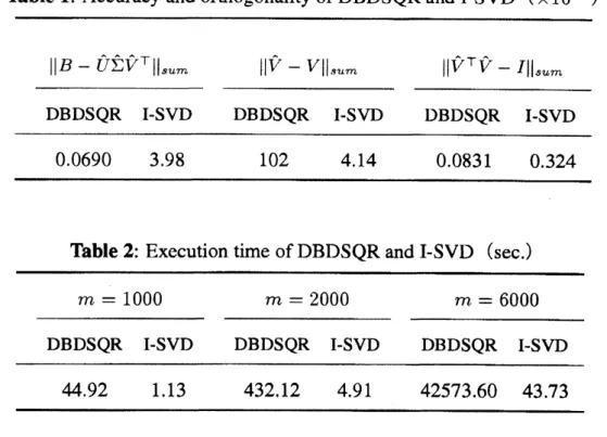
Table

1:

Accuracy and orthogonality of DBDSQRand I-SVD $(\cross 10^{-9})$

$\Vert B-\hat{U}^{\underline{\hat{\nabla}}}\hat{V}^{T}||_{sum}$ $||\hat{V}-V\Vert_{sum}$ $\Vert\hat{V}^{T}\hat{V}-I||_{sum}$

DBDSQR I-SVD DBDSQR I-SVD DBDSQR I-SVD

0.0690

398

102

4.14

0.0831

0.324

Table

2:

Execution timeof DBDSQR and

I-SVD

(sec.)

$m=1000$ $m=2000$ $m=6000$

DBDSQR I-SVD DBDSQR I-SVD DBDSQR I-SVD

4492

1.13

432.12

491

4257360

4373

This is sometimes called thetwisted factorization. The substitution for determining $N(k)$ and

$D^{\pm}(k)$

can

be done from the twisted point _$k=\rho$

as

_$k=\rho,$ $\rho\pm 1,$ $\rho\pm 2$,

. . .

.

While

various

errors

may

be accumulated if

we

compute matrix factorizations by the usual one-side

substitution. The twistedfactorization foreach$\hat{\sigma}_{j}$

can

be computed by$O(m)$ times of divisions.

Since $D_{\rho}e_{\rho}=\gamma e,$ $N_{\rho}e_{\rho}=e_{\rho},$ $D_{\rho}N_{\rho}e_{\rho}=N_{\rho}D_{\rho}e_{\rho},$ _{$v_{j}$} satisfies the linear system $(B^{T}B-$

$\hat{\sigma}_{j^{2}}I)v_{j}=\gamma j,\rho e_{\beta}$ and is

an

eigenvectorof$B^{T}B$ providing that

$N_{\rho}^{T}v_{j}=e_{\rho}$

.

The solution vector$v_{j}=(v_{j}(k))$ of$N_{\rho}^{T}v_{j}=e_{\rho}$ is givenby

$v_{j}(k)=\{\begin{array}{ll}1, (k=\rho),-N(k)v_{j}(k+1), (k=\rho-1, \rho-2, \ldots, 1),-N(k-1)v_{j}(k-1), (k=\rho+1,\rho+2, \ldots, m),\end{array}$

which gives rise to the right singular vector $v_{j}$

.

Since each singular vector

can

be

com-puted within $O(m)$ flops, the computation of k-singular _{vectors costs} $O(km)$ _{flops for} $k=$

$1,2,$ $\ldots,$$m$

.

The left singular vectors $u_{j}$ of $B$

are

given through $U=BV\Sigma^{-1}$, with $U=$ $(u_{1}, \ldots, u_{m}),$ $V=(v_{1}, \ldots, v_{m}),$ $\Sigma=$ diag$(\hat{\sigma}_{1}, \ldots,\hat{\sigma}_{m})$,

or

by solving the system $(BB^{T}-$

$\hat{\sigma}_{j^{2}}I)u_{j}=0$ directly.

Finally

we

quote

some

numerical examples from[301 on

an

_{implementation of theI-SVD}

al-gorithm. InTable 1 the

accuracy

of singularvalue decomposition,the

accuracy

ofrightsingular

vectors and their orthogonality

are

considered. Here $\Vert\hat{V}-V\Vert_{sum}$ indicatesthe

sum

ofabsolute

right singular vectors. The numerical numbers in Table 1

are averages

of

1001000

$\cross 1000$

bidiagonal testmatrices whose singular values

are

randomly distributed. Here DBDSQRis the

standard LAPACK code for bidiagonal SVD where the Demmel-Kahan QR algorithm is

im-plemented. In the I-SVD code the left singular vectors

are

computed by $\hat{U}=B\hat{V}\Sigma^{-1}^{\wedge}$

and

a

re-onhogonalization of all ofthe singular vectors is performed by inverse

iterations

once.

It

takes extra $O(m^{2})$ flops. The parameters $\delta_{\pm}^{(0)}$

are

fixed to 1. Table 1

shows that DBDSQR is

better than the I-SVD code by $1\sim 2$ digits

on

the

accuracy

ofSVD and the _{orthogonality of}

singularvectors. However

on

the

accuracy

of singularvectors I-SVD is betterthan DBDSQR.

Table 2 is a comparison of execution time between DBDSQR and the I-SVD code. It is

obvious that the

I-SVD

algorithm needs only $O(m^{2})$ flops and is rather faster than DBDSQR

of $O(m^{3})$ flops. I-SVD also has

a

better scalability. The I-SVD code with the

Householder

preconditioning to bidiagonal manices and

an

inverse transformation is still sufficiently faster

than DBDSQR with Householder[30].

8.

Concluding

Remarks

This report surveysrecent developmentsofthe mdLVs algorithm for singular values and the

I-SVD algorithm for bidiagonal SVD. The mdLVs is

a

shifted version of the $dLV$ algorithm.

We first show how the $dLV$ algorithm has

a

higher

accuracy.

The Christoffel transformation

of

symmetric OPs

gives

rise to the

positivity

and boundedness of the parameter $\delta^{(n)}$

and the

variable $u_{k}^{(n)}$ of the $dLV$ algorithm. No subtraction

appears

in _$dLV$

.

Positivity

is also essential

in the formulation of the mdLVs algorithm. Namely, if

a

shiftis less than theminimal singular

value, then the positivity of mdLVs follows.

The Johnson bound [171 has been adopted in the mdLVs code [291. Recently

a

new

lower

bound is found which is called the p-th generalized Newton bound. The generalized Newton

shift costs only $O(m)$ flops where $m$ is the size ofgiven bidiagonal matrix [18]. Y. Yamamoto

[19]

proves

that the generalized Newton shiftperfoims

a

weakly $(p+1)$_{-th order}

_convergence.

The mdLVs code with the generalized Newton shift where $p=2,3,4$ is faster and

more

accu-rate than the mdLVs code with the Johnson shift. Though lower and upper bounds of matrix

eigenvalues have been studied fully [311, exploring for

new

bound is still

an

important

problem

in numerical linearalgebra.

The I-SVD algorithm is

a

combination of_{the mdLVs algorithm and the dLV-type}

transfor-mation for singularvectors. Because ofthe separation ofcomputation of singular values from

that of singularvectors theI-SVD algorithm

runs

in $O(m^{2})$ flops. Whereas theDemmel-Kahan

QR algorithmrequires $O(m^{3})$ flops. Thus theI-SVD code is ratherfasterthan DBDSQR code

ofLAPACK. TheI-SVD code has a good orthogonalityofsingularvectors for the

case

of

ran-dommatrices. Toimprove the orthogonality for clustered

matrices

theI-SVD algorithm should

参考文献

[1] N. I. Akheiezer, The ClassicalMoment Problem andSome Related Questions inAnalysis,

Edin-burgh: Olver&Boyd, 1965.

[2] T. S. Chihara,AnIntroduction to Orthogonal Polynomials, New York: Gordon&Breach, 1978.

[3]

$pearMoody$ T. Chu, “Linearalgebra algorithms as dynamicalsystems,

‘’

Acta Numerica, 2008, to

ap-[4] J. Demmel,AppliedNumerical Linear Algebm, Philadelphia: SIAM, 1997.

[5] I. S. Dhillon and B. N. Parlett, Orthogonal eigenvectors and relativegaps, SIAM J. Matrix Anal. Appl.,25(2004), 858-899.

[6] I. S. Dhillon and B. N. Parlett, Multiple representations to compute orthogonal eigenvectors of

symmetrictridiagonalmatrices,_{Lin. Alg. Appl.,}387(2004), _1-28.

[7] I. S. Dhillon, B. N. Parlett andC. Vomel, Gluedmatrices andtheMRRR algorithm, SIAM J. Sci.

Comput., 27(2005),496-510.

[8] K. V. Femando, B. N. Parlett, Accurate singular values and differential qd algorithms, Numer.

Math.,67(1994), 191-229.

[9] G. H. Golub and C. F. Van Loan, MatrixComputations 3rd$edn$_, Baltimore: The _{Johns Hopkins}

Univ. Press, 1996.

[10] R. Hirota, ”Conservedquantities of random-time Todaequation”, J. Phys. Soc.JapanVol. 66, pp.

283-284, _1997.

[11] M. Iwasaki and Y.Nakamura,“Onaconvergenceof solution of the discreteLotka-Volteirasystem;’

InverseProblems, vol. 18,pp. 1569-1578, _2002.

[12] M.Iwasaki and Y. Nakamura,“Anapplicationofthe discreteLotka-Volterrasystem withvariable

step-size to singular value computation,” InverseProblems, Vol. 20,pp. 553-563, 2004.

[131 M. Iwasaki and Y. Nakamura, “Accurate computation of singular values interms of shifted inte-grableschemes, ”

JapanJ. Indust.Appl. Math. Vol. 23,pp.239-259, 2006.

[14] M. Iwasaki and Y.Nakamura, ”Positivity and stability ofthe $dLV$algorithm for_{computing matrix}

singularvalues,”in:Proceedings

_of

the 2nd Intemational

_Conference

on

_Informatics

Research

_for

Development

_of

KnowledgeSociety

_{Infrastructure}

ICKS2007, $Eds$. M. Fukushima, K. Tajima _and

K. Tanaka, IEEE Computer SocietyPress,pp. 103-110,_2007.

[15] M. IwasakiandY. Nakamura, ”Center manifold approachtodiscrete integrable systemsrelatedto

eigenvalues and singularvalues,’‘Hokkaido Math. J., Vol. 36,pp. 759-775, 2007.

[16] M.Iwasaki,_{S. Sakano}andY. Nakamura, ‘Accuratetwistedfactorizat\’ionof realsymmetric

tridiag-onalmatrices and its applicationtosingular valuedecomposition,” Trans. Japan SIAM, 15(2005),

461-481. (岩崎雅史. 阪野真也, 中村佳正, 実対称3重対角行列の高精度ツィスト分解とその

特異値分解への応用, 日本応用数理学会論文誌).

[17] C. R. Johnson, ‘A Gersgorin-type lowerbound for the smallest singular value;‘ $Lin$

.

Alg. Appl.,

Vol. 112,pp. 1-7, 1989.

[18] K.Kimura, T.Yamashita and Y.Nakamura,“On$O(N)$formulaforthe_{diagonalelementsofinverse}

powersofsymmetric positivedefinitetridiagonalmatrices,’‘ inpreparation.

[19] K. Kimura,Y Yamamoto,M. TakataandY Nakamura,_{“Generalized Newton shifts: An arbitrarily}

high ordershufting scheme for singular value computation,” inpreparation.

[21] Y. Nakamura, ‘A new approach to numerical algorithms in terms of integrable systems,”

in:Proceedings

_of

Intemational

_Conference

on

_Informatics

Research

_for

Development

_of

Knowl-edge Society

_{Infrastructure}

ICKS 2004, $Eds$

.

$T$ Ibaraki, T Inui and K. Tanaka, IEEE Computer

SocietyPress,pp. 194-205,2004.

[221 Y. Nakamura, Functionality

_of

Jntegrable Systems, Tokyo: Kyoritsu Shuppan, 2006, (中村佳正著

「可積分系の機能数理」 共立出版).

[23] B. N. Parlett and I. S. Dhillon, Femando’s solution to Wilkinson’s problem: An application of doublefactorizatio$n$,Lin. Alg. Appl., 267(1997),247-279.

[24] B. N. Parlett and $0$

.

A. Marques, An implementation ofthe dqds algorithm (positive _case), Lin.

Alg. Appl.,309(2000),217-259.

[25] H. Rutishauser. “Ein Quotienten-Differenzen-Algorithmus,” $7_{\wedge}$ angew Math. Phys., vol.

5. pp.

233-251, _1954.

[26] V. $Sp\ddot{m}donov$ and A.Zhedanov, ”Discrete-time Volterra chaina$nd$classical orthogonal

polynomi-als,”J. Phys.$A$, vol. 30,pp. 8727-8737, 1997.

[27] G. Szeg\"o, OrthogonalPolynomials, Providence: Amer. Math. Soc., 1939.

[28] M. Takata, M. Iwasaki, K. Kimura and Y. Nakamura, “Implementation and its evaluation of

rou-tine for computing singularvalues with high accuracy,” IPSJ Trans. Adv. Comput. Systems, 46, No SIG12(2005),299-311,(高田雅美, 岩崎雅史, 木村欣司, 中村佳正, 高精度特異値計算ルー

チンの開発とその性能評価, 情報処理学会論文誌).

[29] M.Takata,M. Iwasaki, K.Kimura and Y.Nakamura. “Anevaluationofsingular value computation

by the discrete Lotka-Volterra system,” in:Proceedings

_of

The 2005 Intemational

_Conference

on

Paralleland DistributedProcessing Techniques and Applications (PDPTA2005), Vol. II,pp.

410-416,2005.

[30] M. Takata. K. Kimura. M. IwasA and Y. Nakamura, “Implementation oflibrary for high speed

singular value decomposition2”IPSJTrans. Adv.Comput.Systems, 47, No.SlG7(ACS 14), (2006),

91-104,($\ovalbox{\tt\small REJECT}$ffl%$\not\equiv$, $*\}\backslash \dagger I\overline{\text{ロ}}\urcorner,$ $\epsilon ur\ovalbox{\tt\small REJECT}\Re R,$ $\mathfrak{c}P\}\backslash \dagger\dagger\not\leqq iE$,

-$\ovalbox{\tt\small REJECT}$I $\grave$

ま$*$g{F9$\beta\not\in$のためのライブラ $\dagger$

) $\ovalbox{\tt\small REJECT}$ $\mathfrak{X},$ $’\ovalbox{\tt\small REJECT}\Re\infty g_{\mp\hat{=}p|wX_{\overline{p}}^{-}T)}^{r^{\backslash }3a}$

.

[31] R. Varga,GerSigorinand HisCircles, Heidelberg: Springer-Verlag,2004.

[32] T.Yamashita, K.Kimuraand Y.Nakamura, “Onsubtraction free formulaforthe diagonalelements