微小振動子の入力場位相揺らぎに対するロバストフィルタリング及びLQG制御 (高次元量子トモグラフィにおける統計理論的なアプローチ)

微小振動子の入力場立相揺らぎに対するロバスト

フィルタリング及び

_LQG

$\ovalbox{\tt\small REJECT}\iota$

」

御

慶磨義塾大学大学院理工学研究科 $*$

飯田 早苗

Sanae Iida

Graduate School of

Science

and Technology

Keio University

The quantum Kalman filter and LQG controller provides enough specification for

accurate estimation and control in linear quantum system, though this holds only in the case when a trustful mathematical model of the system is available. In this

paper, we consider an optomechanical oscillator which is continuously monitored via

an

optical laser, although the laser phase is unknown. For this system,

we

propose

a

robust scheme ofboth filtering andcontrol against the phase uncertaintyoftheoptical laser. The filter estimates the uncertain parameter using

an

auxiliary estimator that adaptively changes the filtering and control algorithm

so

that it aquires the better

estimation and control performance

near

to that of the optimal

one.

The robustness

is demonstrated in

a

numerical simulation.

1

Introduction

To realizevarious nano-architectures including quantum informationprocessors [9],

we

needaccurate measurement and control of thesystem under consideration. Quan-tum filtering theory [2, 3, 4] and its application to quantum feedback control [13, 14]

serve

basic methodologies satisfying these requirements and have actually shown the potential usefulness [1, 6, 11]. For linear quantum systems, especially, the filter and

the controller have completely the

same

form

as

the traditional Kalman filter and

LQG controller, thus such a quantum Kalman

_filter

and

a

quantum $LQG$ controller

are

enough implementable in reality.

However,

as

in the classical

case

(we here call “classical only because they are not

quantumsystems), the quantumKalman filter and the quantum LQG controller work well only when a trustful mathematical model of the system under consideration is

available. Fortunately, for this long-standing issue, the classical system theory has

provided

a

number ofsolutions; they

are

largely classified to two approaches.

The first is based

on

the notion of “soft sensing that is, the estimation algorithm

is modified, without adding a real sensor,

so

that the filter and the controller acquire robustness against the model uncertainty [8, 10].

The second is the “hardwaresensing” method that simply introduces actual

sensors

so

as

to obtain

more

information utilizable forthe better estimation under uncertain-ties. This method is, classically

more or

less,

never

inferior to the above soft sensing technique, if one affords to buy an expensive high-quality sensor required. In the

quantum case, however,

we

cannot always have such

a

hopefulstatement. This is due to the unavoidable quantum back-action property; that is, introducing a hardware

sensor

must bring additional noise to the system, thus it sometimes happens that the estimation performance getsworse. The hardware sensingmethod for robust quantum

filtering and control has, presumably because of this fact, not yet been examined.

In this paper, despite of the back-action issue mentioned above, we apply the idea of hardware sensing to the quantum

case

and propose a new configuration of the

quantum Kalman filter and the quantum LQG controller that has robustness against

a certain practical uncertainty.

Let

us

first describe the uncertainty

we

treat in this paper. Fig.1 depicts

a

gen-eral linear quantum system coupling with

an

optical laser field. The output light is measured using so-called balanced homodyne detector, and the signal generated is then processed in the filter to calculate the estimate of the system variable. Also

we can control the system with the estimate

so

that the system has nice property.

In reality,

an

uncertainty appears in this input laser field; that is, the phase of the

input laser cannot be determined in any real experiment. As shown later on, the

phase uncertainty is explicitly contained in all the system, the filter and the

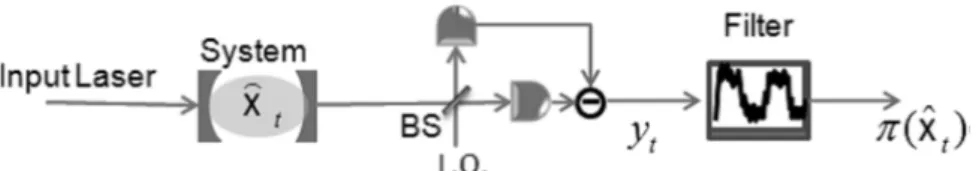
図1 _{Schematic of the} quantum Kalman filter. First, the system couples with a

input laser. Theoutput laser ismixed, byabeamsplitter(BS), withastrong

ref-erence lightcalled the local oscillator(LO), and twooutputs arethen respectively

detected via aphoton detector. This whole measurement configuration is called

the homodyne detection. Finally, the quantum Kalman filter uses the output to calculatethe best estimation $\pi(\hat{x}_{t})$.

control performance. It should be mentioned that this sort of indirect measurement

scheme through

a

laser is commonly used for various quantum systems, for instance

an

atomic system in the cavity QED setup [5, 7] and

an

opto-mechanical system in

an optical interferometer [12]. In this sense, the robust Kalman filtering and LQG control technique under the phase uncertainty of the input laser should be widely

useful and significant.

We next mention briefly about the hardware sensing scheme for robust Kalman

filtering and LQG control. This is built up by first dividing the input laser before it

goes into the system and then putting another homodyne detector along the second

optical path to obtain further information;

see

Fig. 3 in Section 3. $A$ (probabilistic)

back-action is brought when

one

does this additional measurement. Nonetheless,

the hardware sensing scheme proposed allows us to estimate the unknown parameter itself; the result can then be fed back to adaptively change the filtering and control algorithm and, eventually, the filter and the controller acquire robustness property despite of the back-action mentioned above. We call this scheme the adaptive Kalman

filter

and the adaptive $LQG$ controller.

This paper is organized

as follows.

In Section 2, the standard quantum Kalman filter and LQG controller

are

described by taking an opto-mechanical oscillator

as

a system, then the uncertainty issue is explained. Section 3 is devoted to show the

configurationand the algorithm ofthe adaptive Kalman filter andLQG controller. Its

robustness property is further given. Finally, inSection4, wenumericallydemonstrate

図2Schematic ofthe optomechanical oscillator. The right end mirror of the Fabry-Perot cavity serves asthe oscillator, where$\hat{x}_{t}$ is the system variable, $\^{a}_{t}$ is an annihilationoperator corresponding to the intra-cavity, and $\mathcal{A}_{in}$ is the mean

amplitude ofthe input laser.

2

The

quantum

Kalman

filter and

LQG

_controller

The system

we

focus

on

is

an

optomechanical oscillator. Consider now a Fabry-Perot cavity composed of a moving mirror which interacts with an input field $A_{in_{t}}.$

The mirror is modeled with position operator $\hat{q}_{t}$, momentum operator $\hat{p}_{t}$,

mass

$m,$

and resonant frequency $\omega_{m}$

.

The intra-cavity optical field \^a decays at rate $\gamma$ due to

coupling through the partially transmitting mirror to the output beam $A_{out_{t}}$

.

The

intra-cavity opticalfieldassumed to be resonant at theinput beam’s carrier frequency $\omega_{0}$, at which point the roundtrip length is $2L$

.

The mirror position$\hat{q}_{t}$ isdefinedrelative

to this equibirium position. The operators obey canonical commutation relations:

$[\hat{q}_{t},\hat{p}_{t}]=i\hslash,$ $[\^{a}_{t}, \^{a}_{t}^{\dagger}]=1.$

Removing

mean

fields and defining amplitude and phase quadrature operators for the fluctuations that remain, $A_{in_{t}}=\mathcal{A}_{in}+(\hat{\xi}_{1_{t}}+i\hat{\xi}_{2_{t}})$, $A_{out_{t}}=\mathcal{A}_{in}+(\hat{\eta}_{1_{t}}+i\hat{\eta}_{2_{t}})$,

and $\hat{a}_{t}=\alpha+\^{a}_{1_{t}}+i\^{a}_{2_{t}}$ where $\alpha=\mathcal{A}_{in}\sqrt{2}/\gamma$, We

can

obtain the system dynamics

with the variable$\hat{x}_{t}=(\hat{q}_{t},\hat{p}_{t},\hat{a}_{1_{t}},\hat{a}_{2_{t}})^{T}$ which is found in a form of so-called quantum

stochastic differential equation:

$d\hat{x}_{t}=A\hat{x}_{t}dt+B(u_{t}dt+d\hat{\xi}_{t})$, (1)

where $u_{t}=(u_{1_{t}}, u_{2_{t}})^{T}$ is the control input, $\hat{\xi}_{t}=(\hat{\xi}_{1_{t}},\hat{\xi}_{2_{t}})^{T}$ is the input laser, $\kappa(\alpha)=\alpha\omega_{0}/L$ is

an

optomechanical coupling strength, and $\alpha=(\alpha_{1}, \alpha_{2})^{T}.$

The output light ofthe system is subjected to the following equation:

$d\hat{Y}_{t}=C\hat{x}_{t}dt+D(u_{t}dt+d\hat{\xi}_{t})$, (3)

$C=HB^{T}, D=\{\begin{array}{ll}-1 00 -1\end{array}\}$ , (4)

where $\hat{Y}_{t}=(\hat{\eta}_{1_{l}},\hat{\eta}_{2_{t}})^{T}$, and $H$ is

a

2-dimentional

row

vector satisfying $HH^{T}=4.$

The outputs commute with each other, i.e., $[\hat{Y}_{t}, \hat{Y}_{s}]=0,$$\forall s,$$t$, thus the sequence of

scalars $y_{t}=\{y_{s} : 0\leq s\leq t\}$ is obtained. For the observer, the variables

can

be

regarded

as

classical random variables, which implies the existence of classical

condi-tional expectations $\pi(\hat{x}_{t})$ $:=\mathbb{E}(\hat{x}_{t}|\mathcal{Y}_{t})$

.

The quantum Kalman filter is the algorithm

that updates the estimates $\pi(\hat{x}_{t})$ depending

on

the measurement outcome $y_{t}$:

$d\pi(\hat{x}_{t})=A\pi(\hat{x}_{t})dt+Bu_{t}dt+(V_{t}E^{T}+F)d\tilde{y}_{t}$, (5)

$\dot{V}_{t}=(A-FE)V_{t}+V_{t}(A-FE)^{T}$

$+2V_{t}E^{T}EV_{t}+BB^{T}-4FF^{T}$_{, (6)}

$E=HC, F=- \frac{1}{4}BH^{T}$, ₍₇₎

where $d\tilde{y}_{t}=dy_{t}-\mathbb{E}(d\hat{Y}_{t}|\mathcal{Y}_{t})$ represents the innovationterm showing the difference

of $dy_{t}$ and the estimate of $d\hat{Y}_{t}.$ $V_{t}$ represents the (symmetrized)

error

covariance

matrix.

To cool the oscillator, it is expected that a feedback controller minimizing the estimated value of the position operator $\hat{q}_{t}$ and momentum operator $\hat{p}_{t}$

.

Because

of the linearity of both the dynamics and the output equation, this requirement is

satisfied with the LQG control. We can construct an optimal control law $u_{t}^{*}$ that minimizes the following quadratic-type cost function:

$J= \langle\frac{1}{2}\int_{0}^{T}(\hat{x}_{t}^{T}Q\hat{x}_{t}+u_{t}^{T}Ru_{t})dt\rangle$ (8)

where $Q\geq 0$and $R>0$represents the penalty for the variables and the controlinput,

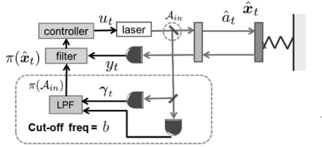
図3Schematic ofthe adaptive quantum Kalman filter and LQG controller.

The LQG control theory gives the explicit form of the optimal controller:

$u_{t}^{*}=-R^{-1}B^{T}P_{t}\pi(\hat{x}_{t})$ (9)

where $P$ is the solution to the following algebric Riccati equation:

彦 $+P_{t}A+A^{T}P_{t}-P_{t}BR^{-1}B^{T}P_{t}+Q=0$ ₍₁₀₎

We here explain the issue of uncertainty. In reality the input laser field amplitude

$\mathcal{A}_{in}=|\mathcal{A}_{in}|(\cos\theta+i\sin\theta)$ is not the value that

can

be determined beforehand. That

is, the phase $\theta$ takes a different value in every experiment and thus should be treated

as an unknown parameter. As shoun in equation (2), $\mathcal{A}_{in}$ explicitly appears in the $A$

matrix (note that $\alpha=\mathcal{A}_{in}\sqrt{2}/\gamma$). Therefore,

we can

never

carry out precise updates

of the estimates, which eventually degrade the total performance ofthe filtering and

control.

3

The adaptive filtering

and

control

We heredescribe the hardware sensing scheme. The input laser is divided into two optical paths via a beam splitter, and the new second path is then measured by the dual homodyne detector. That is, we

measure

both the sine and cosine elements of this second laser field, generating the signal$d\gamma_{t}=\mathcal{A}_{in}dt+dv_{t}$, where$v_{t}$ is

a

2-dimensional

to build the adaptive filter we must introduce vaccum

_fluctuations

that subsequently produce the additional noise $v_{t}$; this is the unavoidable probabilistic back-action

brought by the hardware sensing. The signal $\gamma_{t}$ is then processed through

a

low-pass filter (LPF) with the cut-off angular frequency $b>0$

.

The LPF variable $\pi(\mathcal{A}_{in})$ obeys

$\pi(\mathcal{A}_{in})=e^{-bt}\mathcal{A}_{in_{0}}+b\int_{0}^{t}e^{-b(t-s)}(\mathcal{A}_{in}ds+dv_{s})$

$= \mathcal{A}_{in}(1-e^{-bt})+b\int_{0}^{t}e^{-b(t-s)}dv_{s}$

.

(11)

We find $\mathbb{E}(\pi(\mathcal{A}_{in}))arrow \mathcal{A}_{in}$

as

$tarrow\infty$, thus $\pi(\mathcal{A}_{in})$ asymptotically gives

an

unbiased

estimate of$\mathcal{A}_{in}.$

The adaptive Kalman filter estimates $\hat{x}_{t}$, using the LPF variable $\pi(\mathcal{A}_{in})$ instead

of the unknown parameter $\mathcal{A}_{in}$

.

Writing such

an

estimater

as

$\pi^{A}(\hat{x}_{t})$, the adaptive

Kalman filter and LQG controller

are

given

as

follows:

$d\pi^{A}(\hat{x}_{t})=A^{A}\pi^{A}(\hat{x}_{t})dt+Bu_{t}^{A}dt+(V_{t}E^{T}+F)d\tilde{y}_{t}^{A}$, (12) $u_{t}^{A}=-R^{-1}B^{T}P_{t}^{A}\pi^{A}(\hat{x}_{t})$, (13)

where $A^{A}$ is the $A$ matrix using the LPF variable $\pi(\mathcal{A}_{in})$ instead of the unknown

parameter$\mathcal{A}_{in}$, and $P^{A}$ is the matrix which follows equation (8) using $A^{A}$ instead

of

$A$, and

$d\tilde{y}_{t}^{A}=d\tilde{y}_{t}+E(\pi(\hat{x}_{t})-\pi^{A}(\hat{x}_{t}))dt$

which indicates that the adaptive Kalman filter is driven with

a

difference ofthe true

filter

and the adaptive filter.

$0$ 2 4 6

time 810

図4The difference between the adaptive (or nominal) and the true estimates for $\hat{q}_{t}$

Let

us

here

see

some

actual trajectories of the estimates ofthe adaptive filter and controller. We particularly focus on three types of the filter where the cut-off

fre-quency is chosen as $b=0.5,$$b=0.1$, or $b=0.01$. The true laser amplitude is

$\mathcal{A}_{in}=(1,0)^{T}$, which

can

be used to run the true Kalman filter. For comparison,

we

also examine

a

nominal filter that set $\mathcal{A}_{in}$ to be $(0,1)^{T}$ Fig.4 shows the difference between the adaptive (or the nominal) and the true estimates of $\hat{q}_{t}$

.

We

see

that the

nominal filter fails in the estimation, while the adaptive Kalman filters well estimate, particularly when $b=0.1$

.

Wecannumericallyseethe optimalcut-off frequencywhich

cut-offfrequency

図 5The cut-off frequency dependence of the cost function

minimizes the cost function $J$

.

Fig.5 shows the cut-off frequency dependence of the

cost function. The final time $T$ in this simulation is 3. At lower cut-offfrequencies,

the cost function takes large value. The cost function takes the minimum value at

$b=0.03$, and gradually takes larger value as $b$ get larger. In general, with smaller

valueof$b$, we canobtain morepreciseestimation in the steady state case, but it shows

the more slowly

convergence

to the true filter. In other words, in the early stage of the estimation, the adaptive Kalman filter with small value of $b$ has almost

no

infor-mation of$\mathcal{A}_{in}$, and thus has the

same

quality

as

that of the nominal filter.

On

the other hand, with larger value of $b$, the adaptive Kalman filter has fast convergence,

when

we

take

a feedback

controlwhichrequires rapid convergence and accuracy, there

exists the optimal value ofthe cut-off frequency in terms of the trade-off between the

convergence and the accuracy.

5

Conclusion

In this paper, for an optomechanical oscillator coupling with a laser field, we have

proposed an adaptive filtering and control scheme that estimates both the system

variables and the unknown phase parameter of the input field. It was then shown that, by choosing the cut-offangular frequency in the LPF for the adaptive filtering,

we

can

obtain the robust filter and controller against the phase uncertainty.

Though we have assumed that the uncertainty is constant and only appears in the

phase, inreality these assumptions maynot besatisfied. The robust filteringproblem

in the

more

general setting remains open.

参考文献

[1] C. Ahn, A. C. Doherty, and A. J. Landahl, Continuous quantum

error

correction via quantum feedback control, Phys. Rev. $A$, vol. 65, p. 042301,

2002.

[2] V. P. Belavkin, Quantum filtering ofMarkov signals with white quantum noise,

Radiotechnika $i$ Electronika, vol. 25, pp. 1445-1453, 1980.

[3] V. P. Belavkin, Quantum stochastic calculus and quantum nonlinear filtering, $J.$

Multivariate Anal., vol. 42, pp. 171-201, 1992.

[4] V. P. Belavkin, Nondemolition measurements, nonlinear filtering, and dynamic programming of quantum stochastic processes, in Proc. Bellman Continuum,

$Sophia-Antipoli\mathcal{S}$ 1988,

ser.

Lecture Notes in Control and Information Sciences

121, Springer-Verlag, New York, pp. 245-265, 1988.

[5] H. J. Carmichael, An open systems approach to quantum optics, Springer-Verlag,

Berlin Heidelberg New-York, 1993.

[6] R. Van Handel, J. K. Stockton, and H. Mabuchi, Feedback control of quantum

state reduction, IEEE Trans. Automat. Contr., vol. 50, pp. 768-780, 2005.

[7] H. Mabuchi and A. C. Doherty, Cavity quantum electrodynamics: coherence in

[8] J. B. Moore,

R.

J. Elliott, and

S.

Dey,

Risk-sensitive

generalization ofminimum

variance estimation and control, J. Math. Syst., Estim., Control, vol. 7, pp. 1-15,

1997.

[9] M. A. Nielsen and I. L. Chuang, Quantum Computation and Quantum

Informa-tion, Cambridge University Press, Cambridge,

2000.

[10] I. R. Petersenand A. V. Savkin, Robust Kalmanfiltering

_for

signals and systems

with large uncertainties, Birkhauser, Boston, 1999.

[11] L. Thomsen, S. Mancini, and H. M. Wiseman, Continuous quantum nondemo-lition feedback and unconditional atomic spin squeezing, J. Phys. $B$, vol. 35, _$p.$

4937,

2002.

[12] P. Verlot, A. Tavernarakis, T. Briant, P. F. Cohadon, and A. Heidmann, Scheme

to probe optomechanical correlations between two optical beams down to the quantum level, Phys. Rev. Lett., vol. 102, p. 103601,

2009.

[13] H. M. Wiseman, Quantum theory of continuous feedback, Phys. Rev. $A$, vol. 49,

p. 2133,

1994.

[14] H. M. Wiseman and G. J. Milburn, Quantum Measurement and Control,