The Size Distribution of Firms, Economies of Scale and Growth (Mathematical Economics : Dynamic Macro-economic Theory)

The

Size Distribution

of

Firms,

Economies

of

Scale

and

Growth

Hideyuki Adachi

DepartmentofEconomics,Kobe University,Kobe, 657,Japan

Abstract

The size distribution of firms in each industry$\mathrm{w}\mathrm{i}\mathrm{U}$

$\mathrm{u}\epsilon \mathrm{u}\mathrm{a}\mathrm{I}\mathrm{y}$be highlyskew,and empirical evidence

shows that it is approximated closely by the Pareto distribution. Inthis paperwe makeanattempt to

explain why the Paretolaw applies to the size di tribution offirms basedon their innovation and

investment behavior, and then develop amodel of economic growth that takes into account this

empirical law.First,weshow that the Paretodistributionof firms is generatedunder theassumption

that firms acquire the technology of operating efficientlyonalarger scale through learning bydoing,

and expand theirscaleofoperation through the accumulation ofcapitalinducedbyprofitability.Then,

wesetup amodelof economicgrowththatisbasedontheParetodistributionof firms and economies

ofscale. In our model the growth rate is determined endogenously, and it exhibits scale effects with

respecttosavings and population. Ourmodel isdifferent from the neoclassical growth modelorthe recentlydevelopedendogenous growthmodelsinthatit takesinto accountthesize structure offims,

andit yields quite realstic predictions.

1. Introduction

Empiricallaws

are rare

ineconomics, and

one

of such laws is the regularpattern of

some

statisticaldistributions, such

as

the distribution of personsaccordingto the level

of income

or

of business firms accordingto

some

measurementofsize such

as

sales

or

the number of workers. Manyof these distributions conform tothe $\infty\cdot \mathrm{c}\mathrm{a}\mathrm{U}\mathrm{e}\mathrm{d}$thelawof

Pareto. Many economists attempted to explain the mechanisms that generate the

Pareto distributions by $\mathrm{c}\mathrm{o}\mathrm{n}\mathrm{s}\mathrm{f}\mathrm{f}\mathrm{u}\mathrm{c}\dot{\mathrm{h}}\mathrm{n}\mathrm{g}$ models with stochastic processes. Simon (1955),

Champernowne (1953),Wold and Whittle (1957), _Steindl (1965), etc. maybe mentioned

as

pioneersofsuchmodels.The most ingenious modelamong themisthe

one

developed

by Simon (1955), which explains the Pareto distributions based

on

two simple and

meaningful assumptions’

one

is ‘the law ofproportionate

effect

and the other isthe

constancy of

new

entry. When his model is applied to the size distribution offirms,

however, itis not clear how those assumptions

are

related tofirms’ behavior; Besides,

there is

no

work,

as

far

as

Iknow, that make

use

of this interestingempiricalevidence

on the size distribution of firms to analyze macroeconomic problem such

as

economic

growth

or

income distribution.

数理解析研究所講究録 1264 巻 2002 年 122-144

The purpose of this paper is first to explain why the size distribution of firms is

approximated by the Pareto distribution based

on

the innovation and investment

behavior offirms, and secondly to develop

amodel of economic

growth that takesinto

accountthis empirical law.In

our

model

we

assume

that

new

firmsstarttheir operation

from the minimum size, because theylack notonly the necessary know-how to operate

efficiently at larger size but also sufficient finance to start

on

alarge scale. They

gradually acquire the technology of operating efficiently

on

alarger scale through

learning by doing, and expandtheir scale ofoperation through

accumulation

ofcapital

induced by profitability. We show the Pareto distribution of firms is generated under

suchassumptions.

Using this size distribution function and the learning function,

we

set up amodelof

economic growth embodying economies of scale. In this model the growth rate is

determined endogenously, and it exhibits scale effect with respect to savings and

population growth. Ourmodel is different from the Solow growth model

or

therecently

developed endogenous growth models in that it takes into accountthe size structure of

firms.

The paper is organized

as

follows. Section 2reviews the

Simon’s

model and the

generalization of it by Sato. Section 3introduces learning by doing model to explain

growth of firms. Section 4discusses the determination of investment of firms, and

showsthat theParetodistribution is generated through theprocess oflearning by doing

and capital accumulation. In Section 5,

we

constructamacroeconomic model based

on

thePareto lawand thelearning by doinghypothesis, and analyzeincomedistributionin

this model. Iri Section 6,

we

extend it to agrowth model. Section 7analyzes the

steady-state properties of this model. It is shown that the steady growth equilibrium

exhibits scale effect, but it is unstable. In Section 8,

we

consider the substitutability

between capital and labor, show that the steady growth equilibriumbecomes stable in

that

case.

2. The Size Distribution

of

Firms

The size distributionsoffirms in$\mathrm{U}.\mathrm{S}$

.

and Germany

are

illustratedin theAppendixof

Steindl’s

book (1965). 1 _{They approximate the} Pareto distribution, especially in the

upper tail, whichis givenby

$N(k)=Ak^{-\rho}$

.

(2.1)

Here, $k$ represents the size of firms, $N(k)$ the number of firms with the size in

excess

of $k$,and

$\rho$iscalled the Pareto coefficient. The size of firmsismeasuredbysales,

capital

or

employment dependingontheavailabilityof data. The aboveequation impli

es

thatthe number offirmswith the sizein

excess

of $k$,plotted against $k$ onlogarithmic

paper, is astraightline. The size

distribution

of

firms

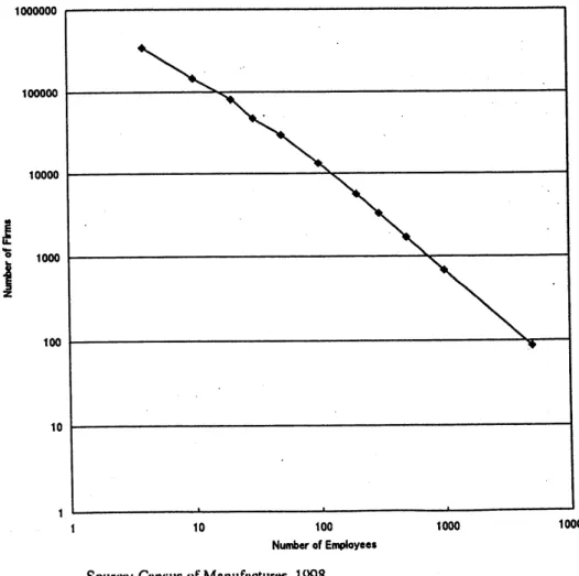
in the Japanese manufacturing

industry,

_as

shownby Fig.1, _{is also}

_{beautiful illustration}

_{of the}

_Pareto

_law.

_It

_is

_almost

entirely astraight

line

on

thelogarithmicpaper.2

The

Pareto distribution

is observed notonly in the size

distribution

of firms butin

many other fields, such

as

distributions of

income

by size,

_{distributions}

_of

_scientists

_by

number$\mathrm{o}.\mathrm{f}$paperspublished, distributionsof cities by

population. 3 _{Whysucharegular}

pattern isobserved in many fields isabigpuzzle.Many_{economists have challenged to}

reveal this puzzle. Among them, the

solution

given by

Simon

(1955)

_seems

_to

_me

_the

simplestand themostingenious.

Let

us

first review the

Simon’s

model. His model

was

designed for anon-economic

problem, namely the distribution ofwords in abook. Suppose _that

_we

_read abook,

classifying words that appear successively.

Some

words appear

more

often than others.

Le.

$\mathrm{t}$the total

number of words in

a

bookalready

run

throughreached $K$

.

We designate

by $f(k,K)$ _{the number of different words that have appeared} $k$ times. Then,

we

musthave

$\sum_{k\cdot 1}^{K}ff(k,K)=K$

.

_(2.2)

Now, Simonmakesthefollowingtwoassumptions’

Assumption 1:The probability _{that the} $(K+1)- st$_{word is aword that has already}

appeared exactly $k$ times isproportionalto _$ff(k,K)$

–thatis, _{to the total number}

of

occurrence

ofall the words thit have appearedexactly $k$ times.

Assumption

There

is aconstantprobability, $\alpha$

.

that the $(K+1)- st$wordbe

anew

$\mathrm{w}\mathrm{o}\mathrm{r}\mathrm{d}\neg$

word that has not occurred in thefirst $K$ words.

The first assumption iscalled the law ofproportional effect, which

was

proposed by

Gibrat (1930) _{toderive the log-normal}

_{distribution.}

_{With this assumption, the expected} number of words that would have appeared $k$ times after the _{$(K+1)- st$}word

has

been drawn isdeterminedby

$E[f(k,K+1)]=f(k,K)+L(K)\{(k-1)f(k-1,K)-\psi(k,K)\}$ , $k=2,\cdots,K+1$

(2.3) where $L(k)$

i.\S

the _{proportionalty factor of the probabilities. The second assumption}

implies _{that the} probability of

anew

entry of aword is constant. This assumption

togetherwith the first

one

givesthe followingequation:

$E[f(1,K+1)]=f(1,K)-L(K)f(1,K)+\alpha$

_.

_(2.4)

Simon

is concerned with “steady-state” distributions,

so

he replaces the expected

values in the above two equations by the actual ffequencies. In other words, the

expectationoperator $E$ isdroppedfrom(2.3)and(2.4) inordertohave the steady state

distribution. Thedefinitionof thesteady-statedistribution is givenby

$\frac{f(k,K+1)}{f(k,K)}=\frac{K+1}{K}$ for all $k$ and

K.

(2.5)

This

means

that all the fiequencies grow proportionately with $K$, and maintain the

same

relative size. The relativefrequencies

denoted

by $f^{*}(k)$ may be

defined

as

$f.(k)= \frac{f(k,K)}{\alpha K}$, (2.6)

where $\mathrm{a}\mathrm{K}$ isthe total number ofdifferentwords.

With the above assumptionsand the definition of thesteady-state distribution,

Simon

shows that the relativefiequencyofdifferent words in the steadystate, which is denote

by $f\cdot(k)$, isindependentof $K$, andbecomes

as

$f \cdot(k)=\frac{(k-1)(k-2)\cdots 2\bullet 1}{(k+\nu)(k+\nu-1)\cdots(2+\nu)}f\cdot(1)=\frac{\Gamma(k)\Gamma(\nu+2)}{\Gamma(k+\nu+1)}f\cdot(1)$ (2.7)

Here,

$\nu=\frac{1}{1-\alpha}$, $f^{*}(1)= \frac{1}{2-\alpha}$ (2.8)

The expression (2.7) _is

_a

$\mathrm{s}\mathrm{t}\mathrm{e}\mathrm{a}\mathrm{d}\mathrm{y}\cdot \mathrm{s}\mathrm{t}\mathrm{a}\mathrm{t}\mathrm{e}$solution to equations (2.3) and (2.4), since it

satisfiesthe latter twoequationswithout theexpectation operator $E$

.

Simon calledthe

expression(2.7)_{the Yule distribution.}

Fromthewell-knownasymptotic propertyoftheGammafunction,

we

have

$\Gamma(k)/\Gamma(k+\nu+1)arrow k^{-(\nu+1)}$

as

$karrow\infty$

.

(2.9)

Hence, from (2.7),

_we

have

$f\cdot(k)arrow\Gamma(\nu+2)f\cdot(1)k^{-(\nu+1)}=Ak^{-(\nu+1)}$

as

$karrow\infty$

.

(2.10)

We

can

confirm that $f.(k)$ _{is aproper distribution function. For}

we

have

$\sum_{k=1}^{\infty}ff.(k)arrow\Gamma(\nu+2)f\cdot(1)\sum_{k=1}^{\infty}k^{-\nu}$, (2.11)

andthisexpressionisconvergentif $\nu>1$

.

Thus,

as

(2.9) shows, the steady state distribution $f\cdot(k)$ obtained under the above

two assumptions is identical with the Pareto distribution for large values of $k$

.

The

value of the Pareto coefficient $\nu$ is determined by the probability of

anew

entry $\alpha$

accordingto (2.8).

It iseasy to interpret

Simon’s

modelexplainedabove in termsof the size distribution of firms. In this context,

we

may interpret $K$

as

the total assets accumulated in the

economy, and$f(k,K)$

as

the number offirmswith assets $k$

.

The parameter $\alpha$ isthe

ratioofthe assetsofnewlyenteringfirms to the increment of assetsofallfirmsabove

a

certain minimum. Thenewly entering

firms

are

ffioae that pass beyond this minimum

intheperiodinquestion. The greaterthe contribution of

new

firms tothe totalgrowth

of assets is, the greater $\mathrm{w}\mathrm{i}\mathrm{U}$ be the Pareto coefficient. The greater Pareto coefficient

implieslessinequalityofthe distribution offirms.

K.

Sato

(1970) _{generalized Simon’s model to include the}

_case

_{where the law of}

proportionate

effect

does not apply.

Instead

of Assumption 1above,

he

assumes

the

following:

Assumption $\mathit{1}’.\cdot$Theprobability thatthe $(K+1)\cdot st$wordis aword that has already

appearedexactly $k$ timesisproportionalto $(ak+b)f(k,K)$ underthe condition that

italso satisfies

$\sum_{\mathrm{b}1}^{K}(ak+b)f(k,K)=\sum_{k=1}^{K}W(k,K)$$=K$

.

_(2.12)

With this assumption together with Assumption 2above, he shows that the

steady-statedistribution becomes

as

$f \cdot(k)=\frac{i^{k+}\frac{b}{a})f\frac{\nu+b}{a}+2)}{?^{k+\frac{\nu+b}{a}+1})}f\cdot(1)$

.

(2.) 1)

Here, $a+b>0$ is required for this value to be finite. This distribution becomes

asymptotically

as

follows:

$f \cdot(k)arrow(k+\frac{b}{a})^{\frac{\nu}{\mathrm{n}}1}$

as

_{$karrow\infty$}

.

(2.14)

This is called Pareto distribution of the second kind. This distribution function when

plotted

on

logarithmic paper,isnot exactly astraightline.

However, since l+(b/ak)\rightarrow l

as

$karrow\infty$ for any given value of $b$

la

, the steady

-statedistribution (2.14)_{isasymptotictoPareto distribution ofthefirstkind, thatis,}

$f\cdot(k)arrow k^{\frac{\nu}{a}1}$

as

$karrow\infty$

.

(2.15)

The smaler the value of $b$la, the

more

closelythe steady-state distribution (2.14) is

approximatedby(2.15).

It is shown that $a$ and $b$ mustsatisfythe following relation with $\alpha$:

b

$= \frac{1-a}{\alpha}$

.

(2.16)

Fromthisrelation,it isobviousthat

a

$\geq 1$ according

as

b$\leq 0$

.

(2.17)

Theexpected growth rateof $k$ is proportional to $(ak+b)/k$, thatis,

$E( \frac{\Delta k}{k})=L(K)\frac{ak+b}{k}=L(K)(a+\frac{1-a}{d})$, $k\in[1,K]$ (2.18)

where $L(K)$ is the proportionality factor. The proportionality factor depends

on

the

total number of words $K$

.

Equation (2.18) implies that the expectedgrowjh rate of $k$

increases

or

decreases with $k,\dot{\mathrm{d}}$epending

on

whether $a>1$

or

$a<1$

.

When $a=1$,

the expected growth rate of firms is independent of size. Thus, Sato obtains the

following proposition:

Proposition 1: Under the assumptions 1’ and 2 above, the size distribution is

asymptotictoParetodistribution, andfollowingthree

cases occur.

(a) _The

_case

_{of proportionate growth} ($a=1$ and $b=0$):In this case, the relative

growth rate is independent of size. The Pareto coefficient is $\nu=1/(1-\alpha)$

as

Simon

demonstrated.

(b) _The

_case

ofsize-impeded growth($a<1$ and $b>0$):Inthis case, the growthrate

is stochastically proportional to $a+b$ at $k=1$, and proportionately declines

towards $a$

as

$karrow\infty$.ThePareto coefficient $\nu/a$ exceeds $\nu$

.

(c) _The

_case

of

size-induced

growth ($a>1$ and $b<0$):Inthis case, the growth rate

is stochastically proportional to $a+b$ at $k=1$, and proportionately increases

towards $a$

as

$karrow\infty$

.

The Paretocoefficient $\nu/a$ is lels$\mathrm{s}$than $\nu$

.

3.

Learning by Doing

and

Economies of Scale

In the neoclassical theory ofthe firm, it is

assumed

that the U-shaped curve, LAC,

ilustrated in Figure 2is the long-run average cost

curve

of all firms in aparticular

industry, freely available to all including to potential

new

entrants. It is not by

empirical observation but by the assumption of perfect competition that the theory

requires the long-run average cost

curve

to be U-shaped. If it is U-shaped, the size

distribution offirmsisexpectedto be

anormal

distribution aroundthe optimum size at

which the long-runaverage cost is minimum. But,

as

is shownby many data, the size

distributions offirms inJapan

as

well

as

inU.S. andGermany

are

highlyskewed, being

approximated closely by the Pareto distribution. This implies that the neoclassical

theoryof the firm is inconsistent with empiricalobservations.4

In thissection,

we

develop adifferentmodel offirms, which explains consistentlythe

observed size distribution of firms–the Pareto distribution. Con.sidering that the

Pareto distribution is derivedfromAssumptions1(or 1) _and2above,

_our

modelshould

be consistent with those assumptions. In the context of size distributions of firms,

Assumption l’andAssumption 2maybe

restated

as

follows

Assumption $\mathit{1}’.\cdot \mathrm{W}\mathrm{h}\mathrm{e}\mathrm{n}$ the aggregate stockofcapital

in

the economy;

$K$, is increased

by one, _{the probabilty of afirm with size} $k$ beingexpandedby

one

isproportional

to

$(ak+b)f(k,K)$ _{under the condition that it alsosatisfy}

$\sum_{b1}^{K}(ak+b)f(k,K)=\sum_{k\cdot 1}^{K}ff(k,K)=K$

.

(3.1)

Assumption 2$\cdot$

.

When

the aggregate stock ofcapitalin the

economy,

$K$

, is

increased

by one, the probability ofthis incrementto be apportioned to newly entering firms is

$\alpha$

.

Assumption i’implies

_{that the}

expected growth

of

firms

with

size

$k$ is proportional

to $a+(b/.k)$, while Assumption 2implies that the ratio ofthe capital stockofnewly

entering

fims

to the

increment

of total capiffi is $\alpha$

.

These

parameters _$a$, $b$, $\alpha$ must

satisfy (2.16). _Depending

_on

_{whether $a>1(b<0)$}

_or

_{$a<1(b>0)$, the expected}

growthof

firms increases

or

decreases with size $k$

.

When $a=1(b=0)$, the _expected

rateofgrowthof firms isindependentof their size.

FollowingAssumption

.2, we

assume

that

new

firms starttheir operations from the

minimum size. There

are

two

reasons

tojustifythis assumption. _{The firstisthat}

_new

entrantsdo nothave the necessary $\mathrm{h}\mathrm{o}\mathrm{w}\cdot \mathrm{h}\mathrm{o}\mathrm{w}$to

operate efficiently at largersizes. The

second is that

new

entrants usually cannot

_{have sufficient finance}

to start

on

alarge

scale. But

once

they have acquired the necessary _{technology and} finance, they $\mathrm{w}\mathrm{i}\mathrm{U}$

expectto growin size. Firmswith

same

size donotnecessarily grow atthe

same

rate.

Profitable firmstend to growfaster thanunprofitablefirms.Their eventualgrowth$\mathrm{w}\mathrm{i}\mathrm{U}$

depend

on

successful experience–learning by doing–and _{the accumulation ofprofits,}

both of which take$\dot{\mathrm{h}}\mathrm{m}\mathrm{e}$

.

Most firms believe that there

are

economies of scale to be gained, if they acquire

necessary technology and necessary finance. In order to expand successfuly in size,

however, afirm hasto master technologyofoperatingefficiently

on

alargescale, and it

is through aprocess learningby doing

that

afirm

can

master such technology.

Arrow

(1962) _{formulated amodelof economic growth based}

_on

_{the hypothesisof learning by}

doing. We follow him toexplainproductivity growthoffirms. We

assume

thatlearning

by doing worked through each firm’s investment Specifically,

an

increase in _afirm’s

capitalstockleadsto

an

increasein itsstock of knowledge, and

therefore

toitsgrowthof

productivity. But the rateofgrowthinproductivitymaybe

different

among

firms

even

with the

same

size.

Some

firms improve their efficiency _{better than others.} Thus,

though each firm

follows

adifferent path in learning by doing,

we

assume

that the

learning

function

ofatypicalfirm withcapitalstock $k$ isexpressed

as

folows:

₅

$\frac{l(\kappa)}{k}=\gamma(k)$, $\gamma’(k)<0$,

k

$\in[1,K]$ (3.2)

$\frac{x(k)}{k}=\delta(k)$, $\delta’(k)\geq 0$, $k\in[1,K]$

.

(3.3)

The notations

are as

follows: $l(k)\equiv \mathrm{a}\mathrm{m}\mathrm{o}\mathrm{u}\mathrm{n}\mathrm{t}$of labor used in production by atypical

firm with size $k$, $x(k)$ outputcapacityof atypical firm with size $k$

.

It is

assumed

that $\gamma(k)$ is adecreasing function, while $5\{\mathrm{k}$) is anon-decreasing function. In this

case,

an

expansion of the typical firm with size $k$ definitely leads to

a

reduction in

costsofproductionatanygivenwages and rentalvalueofcapitalgoods, sincethey

save

labor inputper unit

of

output without increasing capital inputper unit of output by

expandingthe size.

To simplfy the analysis without losing reality,

we

will specify these functions

as

follows:

$\mathrm{Y}(\mathrm{k})=ck^{\lambda-1}$, where $0<\lambda<1$, $k\in[1,K]$ (3.4)

$5\{\mathrm{k}$)$=\ovalbox{\tt\small REJECT}^{\mu 1}$ where $\mu\geq 1$, $k\in[1,K]$

.

(3.5)

Then,

we

have

$l(k)=ck^{\lambda}$, (3.6)

$x(k)=dk^{\rho\ell}$

.

(3.7)

Theserelations fitquitewell to the data ofJapanese manufacturing. 6

4.

Profitability

and

Expansion

of

Firms

The incentive of firms to expand arises from the prospect of improving their

profitability by increasingtheir scale ofoperation.The accumulatedprofits

can

be used

for further expansion, either directly

or as

security for raising external finance.

Therefore, the rate ofprofitisakeyvariable

as

the determinants of theexpectedgrowth

rateof firms in each size.Assumingthat thelearningfunction ofatypicalfirm with size

k is givenby(3.4) _and (3.5),

we can

express itsprofitrate

as

follows:

$e(k)= \frac{x(k)-wl(k)}{k}=\frac{dk^{\mu}-wck^{\lambda}}{k}=dk^{\mu-1}-wck^{\lambda-1}$,

k

_$\in[1<K]$

.

(3.8)

Here,

w

denote the wage rate, which is assumed here to be the

same

for any size of

firms.

In reality, the average wage per worker tends to be

an

increasingfunction ofsize of

firm, although not tothe

same

degree

as

decreasesoflaborinput. One

reason

for thisis

that larger firms will usually have

amore

detailed division of labor, with alarger

proportion ofhigher-paid skilled

or

managerial workers. Another

reason

is thattrade

unions

are

usually

more

powerful in larger firms, and maysucceedin extractingpartof

extraprofits created by

economies

of

scale.

Because of these

reasons,

_we

_assume

_that

the average wage per worker increases with size of

firms

as

follow: 7

$w(k)=w(1)k^{\alpha}$_, where $\omega$$>0$, $k\in[1,K]$

.

(3.9)

To simplify the following analysis

we

assume

that $\mu=1$ in equation (3.7). This

assumption isroughly supportedbyactual data.8 _{With thisassumption and (3.8), the}

rate profitofatypicalfirm with size $k$ becomes

as

follows:

$e(k)=d-w(1)ck^{\lambda+\mathrm{n}-1}’$, _$k\in[1,K]$

.

(3.10)

It is obvious ffom this function

_ffiat

if $\lambda$

$+\omega$ $=1$, the rate of profit is constant

irrespective of firm size $k$

.

If $\lambda$

$+\omega$ $\neq 1$,

on

the otherhand, the rate ofprofitincreases

or

decreases

withfirm size $k$, depending

on

whether

$\lambda$

$+\omega$$<1$

or

$\lambda$

$+\omega$$>1.9$

As

is mentioned above, the incentive

of firms

to expand arises

fiom

the prospect of

improvingtheirprofitabilty by increasing their scale ofoperation. So,

we

assume

that

theexpectedrate ofgrowthofatypicalfirm withsize $k$ depends

on

the rate ofprofit

earnedbythatfirm, $e(k)$

.

Forsimplicity,

we

assume

it tobeexpressed by_thefollowing

linearequation:

$E( \frac{\Delta k}{k})=M(K)\{\tau+\xi e(k)\}$_{, $(\tau>0, \xi>0)$}

.

_{$k\in[1,K]$, (3.11)}

where $M(K)$ _{is the}proportionalityfactor thatdepends

on

totalcapital stock, $K$

.

Substituting (3.10)_into(3.11),

_{we can}

expressequation(3.11)

_as

_follows:

$E( \frac{\Delta k}{k})=M(K)[\tau+\xi\{d-w(1)ck^{\lambda+a-1}\}]=M(K)(p-qk^{\lambda+\alpha-1})$ _{, $k\in[1,K]$}

.

(3.12)

Here, $p\equiv\tau+\Psi$ and $q\equiv\phi(1)c$,which

are

positiveconstants.

First, _{consider the}

_case

_where $\lambda$_$+\omega$$=1$

.

In this case, the expected

rate ofgrowth

becomes

as

$\dot{E}(\frac{\Delta k}{k})=M(K)(p-q)$

.

_{$k\in[1,K]$, (3.13)}

where $p-q$ is constant. In other words, the relative growth rate of firms is

independent of size $k$

.

This

case

corresponds to (a) in Proposition 1, and

we

have

Pareto distribution.

Next

let

us

consider the

case

where $\lambda$

$+\omega$$\neq 1$

.

In thiscase,

as

is obvious from (3.12),

theexpected growthoffirms increases

or

decreaseswithsize $k$ depending

on

whether

$\lambda$

$+\omega$$<1$

or

$\lambda$

$+\omega$$>1$

.

In order torelate (3.12) toProposition 1by Sato, let

us

rewrite

equation(3.12)

_as

$E(\Delta k)$ $\mathrm{M}(\mathrm{k})(\mathrm{p}\mathrm{k} qk^{\lambda+\omega})$, $k\in[1,K]$ (3.14)

andlinearize it around $k\cdot$

.

Then,

we

get

$\mathrm{E}(\mathrm{A}\mathrm{k})=M(k)[p(k-k^{*})-(\lambda+a))q(k -k\cdot)]$

$=M(K)(p-q) \frac{p-(\lambda+a))q}{p-q}(k-k^{*})$, $k\in[1,K]$

.

(3.15)

Thisequation

can

be rewritten

as

$\mathrm{E}(\mathrm{A}\mathrm{k})=M(K)(p-q)(ak+b)$, (3.16)

where

$a \equiv\frac{p-(\lambda+\omega)q}{p-q}$, $b \equiv-\frac{p-(\lambda+a))q}{p-q}k$

.

(3.17)

Equation (3.16) implies that the expected increase in assets of afirm with size $k$ is

proportionalto $ak+b$,which isexactlythe

same as

the condition stated inAssumption

i’above. Inaddition,

we

assume

that $a$ and $b$ defined by (3.17) satisfy (2.16). Then,

the value of $k$

.is

determined

as

$k \cdot=\frac{a-1}{m}.$

.

(3.15)

So, $a$ and $b$

are

determinedbytheparameters givenin

our

model.

Comparing the above results with Proposition 1by Sato,

we

get the following

proposition.

Proposition2: Suppose thatnew firms

are

beingborn in the smallest-size class, and

thatthey account for aconstant rate $\alpha$of the growthintotal assets. Suppose also that

atypical firm of each size class masters technology of operating

more

efficiently

on a

larger scale through learning by doing

as

represented by (3.6) _and (3.7), and that its

rate ofexpansion depends

on

the rate ofprofit

as

expressed by (3.11). Then, the size

distribution of firms convergestothe Pareto distribution of the form (2.14). Depending

on

the value of $\lambda+\omega$,

we

can

distinguishthefollowingthree

cases:

(a) _If $\lambda+\omega$_$=1$, then $a=1$ and $b=0$

.

In thiscase, the growth rate isindependent

ofsize, and thePareto coefficientisequal to $\nu=1/(1-\alpha)$

.

(b) _If $\lambda+a$) $<1$, then $a>1$ and $b<0$

.

In thiscase, the growth rate increases with

size, and the Paretocoefficientis less than $\nu$

.

(c) _If $\lambda+a$_{) $>1$}, then $a<1$ and $b>0$

.

In thiscase, thegrowthrate decreases with

size, and thePareto coefficient exceeds $\nu$

.

5.

Determinants

of

Income

Distribution

In the previous sections

we

were

concerned

with the behavior of firms operating

underpotentialeconomies ofscale in

an

industry, and showed that the size distribution

offirms is approximated by the Pareto distribution under quite realistic assumptions

about the technology and investmentbehavior of firms. In this section we willturn to

theanalysisof the whole economy. It is assumedthat, _{when industries}

_are

aggregated,

there

are

persistent _economies of scale

over

the whole range of firm sizes. While

$\mathrm{e}\mathrm{c}\mathrm{o}\mathrm{n}\mathrm{o}\mathrm{m}\mathrm{i}\mathrm{e}\mathrm{s}\backslash$of scalein

one

industrymay belimited, in anotherthey

are

more

extensive,

andtheyextendrightup to thelargest

observed

sizeof

firms

in

some

industry.Thus,

_we

may

assume

thatthe

Pareto function

appliesto size

distribution

of

firms

in the whole

economy.

We also

assume

that the learning

function

of the form describedby (3.6) _and (3.7)_{is stilapplicablewhen}

_we

_{considerthe behavior of the whole economy.}

If

we

assume

that the size distribution of firms is of the

Pareto

form

over

its entire

range,

we

can

express itbythefrequency

function

as

$n(k)=\mu_{k^{-(p*1)}}$, $(\rho>1, A>0)$_{, (5.1)}

where $k$ representsthesizeoffirm measured byitscapital stock, and

$\rho=\nu$

la.

Suppose thatthe minimum size firm has capital stock $k_{0}$, and the maximum size

firm $k_{T}$.Then,the total number

of

firms isgiven by

$N(k_{0},k_{T})=\Gamma 4$$n(k)\ =A(k_{0}^{-\rho}-k_{T}^{-\rho})$

.

(5.2)

$\mathrm{I}\mathrm{f}\mathrm{w}\mathrm{e}|$ denotetheratio of $k_{f}$ to $k_{0}$ by _$m$,

we

have

$k_{T}=mk_{0}$

.

(5.3)

We $\mathrm{c}\mathrm{a}\mathrm{U}m$ ’size ratio’ in the folowing. Using

this notation,

we can

rewrite (5.2)

_as

follows:

$N(k_{0},k_{r})=A(1-m^{-\rho})k_{0}^{-\rho}$ (5.4)

Similarly, the total stock ofcapitalisgiven by

$K(k_{0},k_{T})=’ \iota_{l}k\iota(k\mu=\frac{\rho 4}{\rho-1}(1-m^{1-\rho})k_{0}^{1-\rho}.$ (3.6)

Taking into account(3.6)_and(3.7),

we can

alsocalculate thetotalemploymentand total

output

as

folows:

$L(k_{0},k_{\tau})=\mathrm{f}^{\mathrm{r}_{l(k)n(kw=\frac{\mu_{\mathrm{C}}}{\rho-\lambda}(1-m^{\lambda-\rho})k_{0}^{\lambda-\rho}}}.$ , (5.6)

$X(k_{0},k_{r})= \int_{l_{l}}^{f}x(k)n(k)\ovalbox{\tt\small REJECT}=a\frac{ed}{\rho-\mu}(1-m^{\mu-\rho})k_{0}^{p-\rho}$ (5.7)

We

assume

here that the totaloutput _{is defined} by _{value added. In the folowing,}

_we

deal with the

case

where $\mu=1$

.

In thiscase, (5.7)

becomes

as

$X(k_{0},k_{T})= \frac{\not\simeq d}{\rho-1}(1-m^{1-\rho})k_{0}^{1-\rho}=d\mathcal{K}(k_{0},k_{T})$

.

(5.8)

Suppose that the minimum size firms (or

_we

_{may call them “marginal} firms”) _set

product price with mark-up factor

7on

wage costs. We

assume

thatmarginal firm$\mathrm{s}$

are

under perfect competition,

so

that

7is

determined

at the level that just

covers

capital costs.Then, thereal wagerate ofatypical marginal firm is givenby

$w(k_{0})= \frac{1x(k_{0})}{\sqrt l(k_{0})}=\frac{d}{\beta}k_{0}^{\mu-\lambda}$ (5.9)

We

also

assume

that the average wage per worker rises with size offirms,

_as

isshown

by (3.9). Whenthe minimum size offirmsis $k_{0}$, (3.9)is rewritten

as

$w(k)=w(k_{0})( \frac{k}{k_{0}})^{w}$ (5.10)

All theoriginal entrants into the industry

are

smallenterprise ofminimum size. They

willgrowby improvingtheirtechnology through experience.Assuccessfulfirmsexpand

their scale, they will,

on

the average, be able to reduce their costs by exploiting

economies of scale. As long

as

$\lambda+a$) $<1$ and $\mu\geq 1$ , the larger firms attain

more

favorableprofit marginsthan smaller firms.

From (5.6), (5.7), $(5,9)$and(5.10)the aggregateshareof wagesinvalue addedbecomes

as

$S_{\vee}= \frac{\rho-1}{\beta(\rho-\lambda-a))}\frac{1-m^{\lambda+\mathrm{n}\succ\rho}}{1-m^{1-\rho}}$

.

(5.11)

Thus,theaggregate wage share inthis model is determinedbythe Paretocoefficient$\rho$,

scale parameters $\lambda$

, $\omega$, $\rho$, the size ratio $m$, and mark-up factor,

7.

This theory of

income distribution isquite different from the orthodoxmarginal productivity theory.It

can

be shown straightforwardly that the aggregate wage share depends

on

those

parameters

or

variablesinthefollowingway.

$\frac{\partial S_{w}}{\partial\rho}>0$, $\frac{\partial S_{\nu}}{\partial\lambda}.>0$, $\frac{\partial S_{\nu}}{\partial a)}.>0$ $\frac{\partial S_{w}}{\delta n}<0$, $\frac{\partial S_{\nu}}{\partial\sqrt}<0$

.

(5.12)

6.

Model of Economic Growth with Economies of Scale

In this section,

we

construct agrowth model to examine the dynamics ofaggregate

variables obtained above. Takingthe time derivatives ofequations (5.4), (5.5), (5.6) _and

(5.8),

_{we can}

rewrite them interms of the growthrates

as

follows:

$\hat{N}=\hat{A}+\frac{\rho}{m^{\rho}-1}\hat{m}-\hat{\phi}_{0\prime}$ (6.1)

$\hat{K}=\hat{A}+\frac{\rho-1}{m^{\rho-1}-1}\hat{m}-(\rho-1)\hat{k}_{0\prime}$ (6.2)

$\hat{L}=\hat{A}+\hat{c}+\frac{\rho-\lambda}{m^{\rho-\lambda}-1}\hat{m}-(\rho-\lambda)\hat{k}_{0\prime}$ (6.1)

$\hat{X}=\hat{A}+\hat{d}+\frac{\rho-1}{m^{\rho-1}-1}\hat{m}-(\rho-1)\hat{k}_{0’}$ (6.4)

where $\hat{y}\equiv\dot{y}/\mathrm{y}$for anygivenvariable

$y$.Thus,thegrowth rate of the numberoffirms,

$\hat{N}$

, andthe growthrate ofcapital, $\hat{K}$

,

are

explained bythe shifting rate of the

Pareto

curve, $\hat{A}$

, _{therateof increase in the size}ratio, $\hat{m}$,and the growth

rate

ofthe

minimum

size firms, $\hat{k}_{0}$

.

The growth rate of labor employment, $\hat{L}$

, depends notonly

on

$\hat{A}.\hat{m}$

and $\hat{k}_{0}$ but also

on

$\hat{c}$

.

which represents

the rate ofchange inlabor inputper unitof

capitalcausedby

exogenous

technological change.As is

obvious from

(3.6),

_adecrease

_in

$c$ leads to areduction in labor input per unit ofcapital for every size

classoffirms.

Therefore, $\hat{c}$ represents

technological change affecting _{every size class of}firms, and

normallytakesnegativevalue.

As mentioned above,

_{we assume}

that

new

entrants start their operation _{at the}

minimum size $k_{0}$, and that theproportion $\alpha$of the

increment

in totalcapital, $\mathrm{A}\mathrm{K}$, is

apportionedtothe

new

firms.Inotherwords,

we

have

$\alpha=\frac{k_{0}\Delta N}{\Delta K}$, (6.5)

which is rewritten

as

.

$N \wedge=\alpha\frac{1}{k_{0}}\frac{K}{N}\hat{K}$ (6.6)

Substituting from (5.4) _and (5.5), _{and takinginto accountthe relation $\rho=1/a(1-\alpha)$,}

we

obtain the followingrelationship

between

thegrowthrateofcapital _{and the growth}

rateof the number of

firms:

$\hat{N}=\frac{\rho-(1/a)}{\rho-1}\frac{m^{\rho}-m}{m^{\rho}-1}\hat{K}$

.

(6.7)

Wemusthave $\rho>1/a$,

as

long

as

$\alpha$ is

Positive.

Substituting thisequation

into(6.1),

we can

express the shifting rateof the Pareto

curve as

follows:

$\hat{A}=\frac{\rho-(1/a)}{\rho-1}\frac{m^{\rho}-m}{m^{\rho}-1}\hat{K}-\frac{\rho}{m^{\rho}-1}\hat{m}+f\hat{l}_{0}$ (6.8)

We

assume

thatlabor grows at aconstantrate, $n$, and

we

consider the

case

of full

employment inthefolowing analysis. Thus,

we

have

$\hat{L}=n$

.

(6.9)

$?\mathrm{b}$ complete the model,

we

have to specifythe equationfor the capital _{accumulation.}

We

assume

herethat

a

$\mathrm{f}\mathrm{f}\mathrm{a}\mathrm{c}\dot{\mathrm{b}}\mathrm{o}\mathrm{n}$

$s$

,

ofprofits andafraction

sw

ofwages

are

saved and

devoted

toinvestment, and that $s_{p}$ islargerthan $s_{w}$

.

10 We also

assume

that there is

no

depreciationofcapital. Then, the growthrate ofcapitalisexpressed bythefollowing

equation:

$\hat{K}=\frac{X}{K}[s_{p}(1-S_{w})+s_{w}S_{w}]$ , (6.10)

where $S_{\nu}$

.is

the wage share defined by (5.10). It is adecreasingfunction of $m$

as

is

shownby (5.11),

so we

denote it

as

$S_{\nu},(m)$

.

In viewof(5.8),

we

have $X/K=d$

.

Inthe

following analysis,

we

assume

$d$ to beconstant. Then, equation(6.10)is rewritten

as

$\hat{K}=d[(s_{p}-s_{w})\{1-\cdot S_{w}(m)\}+s_{w}]$, where $s_{p}>s_{w}\geq 0$ and $S_{w}(m)<0’$

.

(6.11)

Thus, the growth rate of capital $\hat{K}$

is

an

increasing function of $m$

.

Denoting it

as

$\hat{K}(m)$ for notationalconvenience,

we

have $\hat{K}’(m)>0$

.

Now,

our

model consists of7equations [$\mathrm{i}.e.,$ $(6.2)$ through (6.4), (6.7), (6.8), (6.9), and

(6.11)$]$

,which includes 7variables $[i.e., N, X, L, K, A, m, k_{0}]$

.

This completemodel

can

be reducedto the system consisting oftwoequations

as

follows. Substituting (6.8) into

(6.2) _yields

$( \frac{\rho-1}{m^{\rho-1}-1}-\frac{\rho}{m^{\rho}-1})\hat{m}+\hat{k}_{0}=(1-\frac{\rho-(1/a)}{\rho-1}\frac{m^{\rho}-m}{m^{\rho}-1})\hat{K}(m)$

.

(6.12)

This equation represents the equilibrium condition for the capital goods market.

Similarly, substituting (6.8)_and (6.9)_into(6.3) yields

$( \frac{\rho-\lambda}{m^{\rho-\lambda}-1}-\frac{\rho}{m^{\rho}-1})\hat{m}+A\hat{k}_{0}=(n-\hat{c})-\frac{\rho-(1/a)}{\rho-1}\frac{m^{\rho}-m}{m^{\rho}-1}\hat{K}(m)$

.

(6.13)

This equation represents the equilibrium condition for the labor market. The system

consistingofequations (6.12) _and(6.13) _{includes two}variables, $m$and $k_{0}$,

so

that itis

acomplete system.

Eliminating $\hat{k}_{0}$ from (6.12) and (6.13),

we

obtain the dynamic equationfor

$.\hat{m}$ :

$\hat{m}=\frac{1}{D(m)}[\Phi(m)\hat{K}(m)-(n-\hat{c})]$, (6.14)

where,

$D(m)= \lambda(\frac{\rho-1}{m^{\rho-1}-1}-\frac{\rho}{m^{\rho}-1})-(\frac{\rho-\lambda}{m^{\rho-\lambda}-1}-\frac{\rho}{m^{\rho}-1})$, (6.15)

$\Phi(m)=\lambda+(1-\lambda)\frac{\rho-(1/a)}{\rho-1}\frac{m^{\rho}-m}{m’-1}$

.

(6.17) It

can

beprovedthat there exists $\overline{m}$ such that

$D(m)>0$ for $m>\overline{m}$

.

(6.17)

The magnitudeof $\overline{m}$ issufficientlysmallcompared

tothe relevant range of $m$,

so

that

we

may

assume

that $D(m)>0$ _always

_holds

_in

our

_model.

11

_The

$\mathrm{f}\mathrm{f}\mathrm{i}\mathrm{n}\mathrm{c}\dot{\mathrm{b}}\mathrm{o}\mathrm{n}$

$\Phi(m)$,

on

the

otherhand,

_has

the

followingproperties.

$\Phi(m)>0$, $\Phi^{\mathrm{t}}(m)>0$

.

(6.19)

Substituting(6.14)_into($(6.12)$ _{andsolving itwithrespectto} $\hat{k}_{0}$,

we

have

$\hat{k}_{0}=\frac{1}{D(m)}[\Psi(m)(n-\hat{c})-\Omega(m)\hat{K}(m)]$, (6.20)

where

$\Psi(m)=\frac{\rho-1}{m^{P^{1}}-1}-\frac{\rho}{m^{\rho}-1}$

.

(6.21)

$\Omega(m)=(\frac{\rho-\lambda}{m^{P^{\lambda}}-1}-\frac{\rho}{m^{\rho}-1})+\frac{\rho-(1/a)}{\rho-1}\frac{m^{\rho}-m}{m^{\rho}-1}(\frac{\rho-1}{m^{r\iota}-1}-\frac{\rho-\lambda}{m^{P^{\lambda}}-1})$

.

(6.22)

It

can

be shown that12

$\Psi(m)>0$, and $\Omega(m)>0$

.

_(6.23)

Thus, equation (6.14) _{determines the dynamic path of} $m$ starting ffom its initial

value. Corresponding to the path of $m$

.

the growth rate of capital $(\hat{K})$ and the

minimum size offirms $(k_{0})$

are

determined.The growthrate ofoutput$(\hat{X})$ isequalto

the growth rate of capital (K) _{under the assumption of fixed}

_coefficient.

_This

assumptionwill be

relaxed

later.

7.

The

Steady

_{Growth and its}

Instability

In this section,

we

examine theproperties of the steady state ofthe above model. In

viewof the dynamic equation(6.14), _{the steady growth equilibrium is attained at} $m$

.

thatsatisfiesthe followingequation:

$\hat{K}(m.)=d[(s_{p}-s_{\nu})\{1-S.(m.)\}+s.]=\Phi(m.)$

n

.

(7.1)

$-\hat{c}$

Since

both $\hat{K}(m)$ and _$\Phi(m)$

are

increasing functions, it is

straightforwardthat arise

inthe savingrate (either $s_{p}$

or

$s_{\mathrm{w}}$)will increase mm, and also the steadygrowthrate

ofcapital, $\hat{K}(m^{*})$

.

In thisrespect,

our

modelis different from the Solowgrowthmodel

inwhich the steady growth rate does notdepend

on

the saving rate. Thisresult

comes

from the fact that, in

our

model, firms with different size grow

over

time by taking

advantageofpotentialeconomies of scalethrough learning by doing. This featureof

our

model may

seem

somewhat similar to theendogenous growthmodel ofthe Arrowtype.

However,

our

modeldiffers from theexisting endogenousgrowthmodels in that it takes

into accountof the size distributionof firms.

We

can

alsoexamine how the steadygrowthisaffectedbythe structuralparameters,

such

as

the Pareto coefficient, $\rho$, the scale effect, /1, the wage structure, $\omega$,

or

mark-upfactor,

_7.Let

us

firstexaminetheeffects ofachange inthe Paretocoefficient,

$\rho$

.

Asis shownby (5.11),

an

increase in $\rho$ leadsto

an

increase in $S_{w}$

.

It

means

that

the wage share function $S_{w}(m)$ inequation (7.1) shiftsupward.Then, the steadystate

value of the sizeratio, $m.$_, mustincrease, since $\Phi(m)$ in equation (7.1) is

an

increase

function. Therefore, the steadygrowth rate ofcapital, $\hat{K}(.m.)$, willdecrease. Note that

the Pareto coefficientis determined by $\rho=1/a(1-\alpha)$, where $\alpha$ isthe share of

new

firms’ investment in the total increment of capital, and $a=1$ , $a>1$ ,

or

$a<1$ depending

on

whether $\lambda+a$)$=1$, $\lambda+\omega$_$<1$

or

$\lambda+a$) $>1$

.

An increase in $\alpha$

or

a

decrease in $a$ brings about

an

increase in $\rho$, which implies higher equality in the

distribution of firms. Thus,

more

equal size distribution leads to the lower wage share

and to the lower growth rate. But it should be noted here that changes in $\rho$ take

a

long periodoftime, since Pareto distribution is the steady-statedistribution.Therefore,

changesin $\rho$ haveeffects

on

variousvariablesonlyafteralong periodof time.

The effects ofachange in /1 _{may similarly be examined. As is shown by} (5.11),

_an

increase in $\lambda$ affects

$S_{\nu}$ to the

same

direction

as an

increase in $\rho$

.

Therefore, it

leadsto thelowerwage shareand to the lower growth rate. An increase in $a$) alsohas

the

same

effectsboth

on

the wage share andthe growth rate.

Conversely,

an

increase in the mark-up factor,

7,

will increase the steady growth

rate of capital, since it shifts the wage share function downwards and leads to

a

decreasein $m$

as

the result.

Next,

we

examinethe stabilityof thissteadygrowth equilibrium. Forthis purpose,let

us

focus

on

equation (6.14). _{It isaone-variable differential}equation, which determines

the timepath of $m$

.

Since $D(m)$, $\Phi(m)$ and $\hat{K}(m)$

are

allincreasing functions, $\hat{m}$

is

an

increasing function with respect to $m$ in the neighborhood

of

the steady state

equilibrium, $m=m.$.Hence, the steady state is unstable. Fig. 3provides agraphical

representation of this instability property. Suppose that $m>m$

.

holds initially. Then,

$m$ and $\hat{m}$ will increase

over

time, and

so

will $K\wedge(m)$

.

In this case, the equilbrium

condition for the labor market(6.13) $\mathrm{w}\mathrm{i}\mathrm{U}$be violated

sooner

or

later, since

we

musthave

$\hat{k}_{0}\geq 0$ when

$k_{0}$ reached its minimumvalue. Conversely, suppose that $m<m$

.

holds

initially. Then, $m$ and $\hat{m}\mathrm{W}\overline{1}\mathrm{u}$decrease

over

time, and

so

will

$\hat{K}(m.)$

.

In thiscase, the

equilibriumcondition for thecapitalgoodsmarket(6.12) _{will beviolated}

_{sooner or}

_later,

since

we

must have $\hat{m}+\hat{k}_{0}=\hat{k}_{T}$ : 0unless the largestfirms shrink they: size. Thus,

the steady growth equilibrium $\mathrm{w}\mathrm{i}\mathrm{U}$ not be maintained, unless

$m=m$

.

is satisfied initially.

E.

Factor

Substitution

and

the

Stability

of the

Steady

State

Equilibrium So far

we

have assumedthat theproductionprocessoffirms with each size ofcapital

is characterizedbyfixedcoefficients,

so

thatafixedamountof labor is used and afixed

amount ofoutputisobtained. In this section,

we

take into account the substitutability

between labor andcapital, and showthatitstabilizesthesystem.

When there issubstitutabilitybetweenlaborandcapital, theproductionfunctionof

a

typicalfirm with size $k$ maybeexpressed

as

$x$$=F$

(

$\frac{\delta(k)}{\gamma(k)}\mathit{1}$, $\delta(k)k$

),

(8.1)

where $\gamma(k)$ and $\delta(k)$

are

thelearningfunctions definedby(3.2) and (3.3).Assuming

that this production function exhibits constant returns to scale and other usual

properties,

we can

rewrite (8.1)

_as

_follows:

$x$$= \delta(k)k\phi(\frac{1}{\gamma(k)}\frac{l}{k})$, where $\phi(0)=0$, $\phi’>0$, $\phi’<0$ . (8.2)

typicalfirm with size $k$ is assumed to make achoice oftechnique tominimize the

totalcost, givenoutputcapacityand technological knowledge.Thus, theproblem of the

typicalfirm isformulated

as

follows:

$\min wl$$+rk$_, $\mathrm{s}.\mathrm{t}$

.

$\overline{x}=\overline{\delta}k\phi(\begin{array}{l}\mathrm{l}l--\overline{\gamma}k\end{array})$ (8.3) Thefirstorderconditionfor this minimizationproblemis

$\frac{w}{r}=\frac{\emptyset’(l/\hslash)}{\phi(l/\gamma 7)-(l/\hslash)\phi’(l/\hslash)}$ (8.5)

Solvingthisequationinwithrespectto

11

$k$,

we

have

$\frac{l}{k}=\overline{\gamma}\psi(\frac{w}{r})$, where $\psi’<0$

.

(8.5)

Let

us

consider the

case

where the learning function $\gamma(k)$ is specified

as

(3.4).

Substituting (3.4)_into (8.5),

_we

have

$l=c\psi(w/r)k^{\lambda}$ (8.6)

This functionreplaces (3.6). _{We also specify the function}$\delta(k)$

as

(3.5), and

assume

$\mu$

to be unity and $d$ to be constant. Underthese assumptions, substitution of(8.6)into

(8.2) _gives

$x$$=d\phi(\psi(\mathrm{u}//r))k$ (8.7)

This function replaces (3.7). Thus, (8.6) _and (8.7) represent the learning process that

takes into consideration thesubstitutabilitybetween labor andcapital.

In

our

model, the wage rate isendogenously determinedby (5.9) _and (5.10), butthe

rateofinterest, is givenexogenously. So,

we

assume

$r$ tobe constant andputitequal

to unity for convenience. In addition,

we

specify $\psi(w)$

as

afunction with constant

elasticity,thatis, $\psi(w)=w^{-\eta}$, where $\eta$ isassumedto be less thanunity.Then, (8.6)is

rewritten

as

$\mathit{1}=cw^{-\eta}k^{\lambda}$ (8.8)

It should be noted here that the wage rate $w$ is afunctionof $k$,

as

isshownby(5.10).

Substitutingthis(8.8)_into (5.6) _andtaking(5.10) _intoconsideration,

we

have

$L(k_{0}, k_{T})= \frac{\rho 4c\{w(k_{0})\}^{-\eta}}{\rho-\tilde{\lambda}}(1-m^{\tilde{\lambda}-\beta})k_{0}^{\tilde{\lambda}-\rho}$

.

(8.9)

Itis$\mathrm{a}\mathrm{s}\mathrm{s}\mathrm{u}\mathrm{m}\dot{\mathrm{e}}\mathrm{d}$here that $\lambda$ _{$=\lambda-\eta a$)}$>0$ .Then, thegrowth rate of the totalemployment

isgiven by

$\hat{L}=\hat{A}+\hat{c}-\eta\hat{w}(k_{0})+\frac{\rho-\overline{\lambda}}{m^{\rho-\tilde{\lambda}}-1}\hat{m}-(\rho-\tilde{\lambda})\hat{k}_{0}$

.

(8.10)

Substituting(8.8)into (5.9),

we

have thefollowingequationthatshows determination of

thewage ratefor marginalfirms.

$w(k_{0})= \frac{1d}{\beta c\{w(k_{0})\}^{-\eta}}k_{0}^{1-\tilde{\lambda}}$ (8.11)

Takinglogarithmicdifferentiationof thisequationand solvingitwithrespectto $\hat{w}(k_{0})$,

we

have thefollowing equation

$\hat{w}(k_{0})=\frac{1}{1-\eta}[(1-\lambda)\hat{k}_{0}-\hat{c}]$ (8.12)

Substituting

this

equationinto (8.10),

_we

_{have the}

_{following equation}

_{for the}

_growth

rateof the totalemployment.

$\hat{L}=\hat{A}+a$$\hat{e}+\frac{\rho-\tilde{\lambda}}{m^{P^{\tilde{\lambda}}}-1}.\hat{m}-(\dot{\rho}-\tilde{\lambda}+\epsilon)\hat{k}_{0’\prime}$ (8.13)

where

$\kappa\equiv\frac{1}{1-\eta}>0$, $\epsilon$$\equiv\frac{\eta(1-\tilde{\lambda})}{1-\eta}>0$ (8.14)

Thus, when

we

take into consideration the factor substitution in

our

model, the

equationfor thegrowthrateof totalemployment(6.3) _{isreplaced by} (8.13).

_{In this}

_case

thedynamicequationfor

firm-size

ratio, (6.14),_isreplacedby

$\hat{m}=\frac{1}{\tilde{D}(m)}$[$\tilde{\Phi}(m)\hat{K}$(m)-(n-a\^e)], (8.15)

where

$\tilde{D}(m)\equiv(\tilde{\lambda}-\epsilon)(\frac{\rho-1}{m^{\mathcal{F}^{1}}-1}-\frac{\rho}{m^{\rho}-1})-(\frac{\rho-\tilde{\lambda}}{m^{\mathcal{F}^{\overline{\lambda}}}-1}-\frac{\rho}{m^{\rho}-1})$ (8.16)

$\tilde{\Phi}(m)\equiv\tilde{\lambda}+(1-\tilde{\lambda})\frac{\rho-(1/a)}{\rho-1}\frac{m^{\rho}-m}{m^{\rho}-1}$ (8.17)

It

can

be shown that if $\epsilon$ is sufficiently large, then $\tilde{D}(m)<0.13$ In this case,

the

dynamic equationfor $m$ hasnegative slope

on

$m-\hat{m}$ plane,

as

is shown in Figure _4.

So,_thesbady-shte equilibriumof thissystemis.stable.

Thecomparative analysisofthe steady state equilibriumthat

we

have carried out in

the last section becomes actually meaningful for the model in this section, _{since its}

stabilityhas beenproved

FOOTNOTES

1.

See

alsoSimon and Bonini (1958).

2. Taking logarithmofequation (2.1) _andregressingit to the size distribution of firms

inJapanese manufacturingindustry

as

shownbyFigure 1,

_we

_{obtain the following}

results:

$\log N=6.38-1.17\log k$ $(R^{2}=0.995)$ (0.06) (0.027)

where the numerical values below eachcoefficientrepresentitsstandard

error.

3. See Simon

(1955)_{for such}examplesof the Pareto distribution.

4. Lydall (1998) _{criticizes the neoclassical theory of firms from this}pointofview, and

proposes

an

alternative theory. Though his ideas presented in his book

are

quite

interesting, he does notpresentany concrete model.

5. The form ofthe function assumed hereisthe

same as

Arrow’s. However,he

assumes

thatthe learning enters atthe production of

new

capital goodsin aggregate, while

we assume

that it enters in the process ofcapitalaccumulation ofeachfirm.

6. Taking logarithm ofthese equations and regressing them to the data ofJapanese

manufacturing industry,

we

obtainthe followingresults:

$\log l=$-0.41+0.83$\log k$ ’ $(R^{2}=0.998)$

(0.04) (0.012)

$\log x$$=0.13+$$0.99\log k$ $(R^{2}=0.999)$, (0.03) (0.009)

where the numerical value below eachcoefficientrepresentsitsstandard

error.

7. Regression of this equation to the data of Japanese manufacturing industry gives

the following result.

$\log w$ $=0.37$\dagger0.08 $(R^{2}=0.968)$

.

(0.02) (0.005)

where the numerical value below each coefficientrepresentits standard

error.

This

resultshows that thepositiverelation between the wagerateand the size offirms is

statisticallysignificant.

8. See the secondregression equationin footnote 5, which shows $\mu=0.99$

.

9. In the

case

of $\lambda+\omega$ _$>1$,thesize of firms will be bounded above

as

follows:

$.k \leq(\frac{w(1)c}{d})^{\frac{1}{1-\lambda-\omega}}$

For,the rateofprofit, $e(k)$, willbecomenegativeunless $k$ satisfiesthisinequality

10. More

orthodoxapproachtothe

determination of

savinginrecentmacroeconomics is

to

assume

that the households maximize

lifetime

utility.

But

it istoo complicatedto

dealwith

our

model by introducingffiisassumption.

11. Weomit theproofto

save

space.

12. We omit theproofto

save

space.

13. We

omit

the

proofto

save

space

REFERENCES

Arrow, K. J. (1962), _{“The Economic Implications of Learning by Doing,” Review of}

EConomicStudies,Vo1.24(June),pp. 155. 13.

Champernowne, D. G. (1953), _{“AModel of}

_Income

_{Distribution,”} $Boelzo\dot{r}c$Jourod,Vol.

63 (June),pp.318-351.

Gibrat, _R. (1930), _{LesInegalites EConomique,}

_{Paris: Librairie}

_{du Sirey.}

Lydall, H. (1998),ACritiqueoftheorthodox Economics,_{Lomdon: Macmillan.}

Sato, K. (1970), “Size, Growth, and Skew $\mathrm{D}\mathrm{i}\mathrm{s}\theta \mathrm{i}\mathrm{b}\mathrm{u}\dot{\mathrm{b}}\mathrm{o}\mathrm{n}^{\mathrm{n}}$,Discussion

Paper, No. 145,

SUNYatBuffalo.

Simon,H. A. (1955), _{“On aClass of Skew}$\mathrm{D}\mathrm{i}\epsilon \mathrm{f}\mathrm{f}\mathrm{i}\mathrm{b}\mathrm{u}\dot{\mathrm{b}}\mathrm{o}\mathrm{n}.$’Biometrics, Vol. 82,pp.

145-164.

Simon, H. A. and Bonini, _{C. P.} (1958), _{“The Size}

_Distribution

_of

_Business

_Firms,”

AmericmEconomicReview,Vol.48(September), pp.607-17.

Steindl, J. (1965), RandomProcessesBpd_{theGrowth ofFirms London: Griffin.}

Wold, H.

0.

A. and Whittle, P. (1957), _{“AModel Explaining the}

_{Pareto Distribution}

_of

Wealth,” EConometrica, _Vol.

25

(October),pp.591-595

Figure

1.

Perfectly

Competitive

Equilibrium of

the

Firm

Figure 2. TheSize DistributionofFirmsinJapanese ManufacturingIndustry

Source:Census ofManufactures,1998.

(Ministryof International Tradeand Industry

Figure

3.

Instability

ofthe

Steady

Growth

Equilibrium

0

Figure

4.

Stability of the Steady

Growth

Equilibrium

0

$m$