Wavelike-particle structures in Boltzmann equation and its applications (Mathematical Analysis in Fluid and Gas Dynamics)

Wavelike-Particle

Structures in Boltzmann

Equation and

its

Applications

Shih-Hsien Yu

Department of Mathematics, National University of Singapore

Abstract

A wavelike-particlelike structure in the Boltzmann equationwasdeveloped since 2002. This developmenthadled tosomequantitative and qualitative analysis inthe nonlinearproblems forthe Boltzmannequation. We willgive abrieflysurveyofthis development. The dual natureproperty givesriseto the precise construction of the Green’sfunction for Boltzmann equation around aglobal Maxwellianstate. By the

precise structure in Green’s function, various problemssuch as invariant manifolds

for the steady Boltzmann flows, time asymptotic nonlinear stability ofBoltzmann shock layers and Boltzmann boundary layers, Riemann Problem, and bifurcation

problem of boundary layer problem, etc. can be analyzed.

1

Introduction

The hard sphere collision model for the Boltzmann equation is:

$\partial_{t}f+\xi\cdot\nabla_{\vec{x}}\mathfrak{f}=Q(f)/\kappa, \mathfrak{f}(\vec{x}, t,\xi)\in \mathbb{R}, \vec{x}, \xi\in \mathbb{R}^{3}, \kappa>0$. (1)

Here, $f(\vec{x}, \xi, t)$ stands for the gas particle velocity density function with velocity $\xi\in$

$\mathbb{R}^{3}$

at $(\vec{x}, t)\in \mathbb{R}^{3}\cross \mathbb{R}$; and $Q$ is a bilinear integral operator on the velocity density

function $f(x, t, \xi)$, which represents the mechanism for particle collision. One can regard

the collisionoperatoras anequilibrating mechanism. The constant $\kappa>0$isthe Knudsen’s

number, which represents the meanfree path of the gas flow.

This equation is a particularly interesting equation in terms of its physics nature by

varying the size of $\kappa$ and the sizes ofthe space-time scales. When $\kappa\gg 1$ and in

a

small

space-time scales, the solution behavior resembles to free particle motions. When $\kappa\ll 1$

and space-time scales

are

large, the balance of the transport nature $\partial_{t}+\xi\cdot\nabla_{x}$ and the

equilibratingmechanics by$Q$ results in aconventional compressible fluid structure, which

is close to the compressible Euler equation for ideal gases by the Hilbert expansion.

With the presence ofaphysical boundary, the gas flows behave very differently from

the conventional fluid mechanics such as the thermal transpiration flows, edge flows,

condensation-evaporation problems, etc. mentioned in the monograph by Sone, [35].

Grad, [9, 8, 10], also recognised an atypical nature when the presence of boundary. He

boundary, initialdata, and shock

wave

which

are

the key elements for adeep

understand-ing ofthe Boltzmannequation.

Since the collision operator $Q$ is

a

nonlinear integral operator, it attracts attentions

of researchers to develop theories

on

$Q$ such

as

the exponentially fast convergence to

an equilibrium state for a space homogeneous problem, [2, 3]. However, those beautiful

results on space homogeneous problems did not provide so much informations to study

the space inhomogenous problems. The first global result

on

nonlinear theorem with the

presence of $\xi\cdot\nabla_{\vec{x}}$ by [36]

was

due to

a

better understanding of the spectral property of

thelinearized Boltzmannequation $(\partial_{t}+\xi\cdot\nabla_{x}-L)g=0$ in [6], where$L$ is alinear collision

operator around a global Maxwellian state. The analysis

on

the spectrum of$-\xi\cdot\nabla_{\vec{x}}+L$

is the first analytic establishment on the balance of$\xi\cdot\nabla_{\vec{x}}$ and L.

The mathematical developments onthe Boltzmann equation thrilled since late 70 by

various groups by different approaches and interests. Mathematically and physically, the

collective behavior among $\xi\cdot\nabla_{\vec{x}},$ $Q$, and a physical boundary is

even

more interesting

and complex. However, one still expects further substantial progress in this regard to

achieve the understanding so that this subject is possible. On the other hand from 60

Sone [22, 23, 24, 24, 26, 27, 28, 29, 30, 31] has obtainedveryinteresting theories regarding

to boundary phenomena related to the Boltzmannequation and kinetic equations.

In year

2002

a completely different approach in the mathematical analysis for the

Boltzmannequation

was

introduced by

Liu

and Yu to

serve

as

aprimarytool to undertake

the analysis for the singular layers

arouse

from the shock layer, boundary layer, and initial

layer as well

as

to give some partial results on Sone’s discoveries. This is an approach

based on the dual physical natures “wavelike-particlelike” of the Boltzmann equation.

This article isaimedtoreviewthis development and its applicationstowardsthe problems

by Sone and Grad.

2

Some

background

and

motivation

for

Boltzmann

equation and

conservation

laws

In [6],

one

considers the spectrum problem

$(-i\xi\cdot\eta+L)\psi(\eta)=\sigma(\eta)\psi(\eta)$ (2)

for the linear Boltzmannequation

$f_{t}+\xi\cdot\nabla_{\vec{x}}f-Lf=0$ (3)

around a global Maxwellian state $M=M_{[1,0,\theta]}$ in the Fourier variable $\eta\in \mathbb{R}^{3}$, where

$M_{[\rho,u,\theta]}(\xi)=\rho\frac{e^{-1*^{-u}L^{2}}}{(4\pi\theta)^{3/2}}$

$|\eta|<\kappa_{0}$ there

are

five branches $\sigma_{j}(|\eta|)\subset\{z\in \mathbb{C}|Re(z)<0\}$ tangential to the imaginary

axis with the asymptotic for $|\eta|\ll 1$

$\{\begin{array}{l}\sigma_{1}(\eta) , \sigma_{2}(\eta)=\pm ic|\eta|-A_{1}|\eta|^{2}+O(|\eta|^{3}) ,\sigma_{j}(\eta)=-A_{j}|\eta|^{2}+O(1)|\eta|^{3} for j=3, 4, 5,\end{array}$ (4)

with $A_{j}>0$, where$c=\sqrt{5\theta}/3$ is the speed of sound

wave

at rest; and there is aspectral

gap:

$\sigma(\eta)\not\in\{Re(z)>-\kappa_{1}\}$ for $|\eta|>\kappa_{0}$. (5)

One can view the spectrum $\sigma(\eta)$

as

a balance of the space transport mechanism $\xi\cdot\nabla_{\vec{x}}$

in the Fourier variable $\eta$ and the linear collision operator L. By this spectrum property

in [36],

one

applied a resolvent approach and a bootstrap approach to yield nonlinear

stability ofa global Maxwellian state M.

In [11, 21], one expanded the eigenfunction $\psi(\eta)$ in terms of the collision invariants

of $L$ so that the relationship between the Boltzmann equation and the hydrodynamic

equations is clearer. The expansion of the eigenfunctions gave hints to the introduction

of macro-micro decomposition in [14]:

$f=P_{0}\mathfrak{f}+P_{1}\mathfrak{f}\equiv \mathfrak{f}_{0}+f_{1}$, (6)

where $P_{0}$ is a linear combination of finite number of collision invariants related to a

local Maxwellian; and one can identify $f_{0}$

as

a vector in $\mathbb{R}^{3}$

for a planar wave problem.

With this decomposition, one can rewrite the time asymptotic stability for aplanar

wave

perturbation $j,$ $\partial_{t}j+\xi^{1}\partial_{x}j=\frac{\delta Q}{\delta\varphi}j+Q(j)$, of a Boltzmann shock profile $\varphi$ coupled with a

$3\cross 3$ viscous systemthrough the microscopic component$j_{1}$ of$j$:

$\partial_{t}F+A(x)F_{x}=B(x)F_{xx}+O(1)J(\partial_{t}j_{1}) , F\in \mathbb{R}^{3}$. (7)

Here, the Boltzmann shock profile $\varphi$ of(1) is atravellingwavesolution $f(x_{\}}t)=\varphi(x-st)$

connecting two Maxwellians $M_{[\rho\pm,u\pm,\theta\pm]}$ given by a hyperbolic shock wave $((\rho-,$$u_{-},$$\theta$

$(\rho+, u_{+}, \theta_{+}))$ together with the speed $s$ given the Rankine-Hugoniot condition.

Then, by assuming that the difference of the end states of the shockwave is sufficient

small and the total macroscopic component of perturbation is zero, one shows that the

Boltzmann shock profile is stable by implementing the energy method for conservation

laws by [7]. The consequence of the stability is that the Boltzmann shock profile $\varphi(x, \xi)$,

obtained by [1], is a positive-valued function in $(x, \xi)$.

With the micro-macro decomposition, one can implement this energy method to work

out the problemabout the existence of Knudsen layers (boundary layers) with condition,

$|MachNumber|\neq 0$,1, [37]. Theenergymethod

was

also applied to derive

a

macroscopic

[18], and to show nonlinear stability of the boundary layer with Mach number less $-1,$

[38]. When Mach Number $>-1$, the energy method

can

not be applied due to the fact

that the solution of initial boundary value problem contains singularity at boundary

so

that the energy method could not be applied. It led to search for a new approach which

does not require regularity property of the solution. The right candidate for such a tool

is the Green’s function since the Boltzmann equation is

a

semilinear equation.

3

Particlelike-Wavelike

Duality

One starts to consider problems in planar wave solutions to establish the understanding

on the natures ofthe Boltzmann equation, i.e. $x,$$\eta\in \mathbb{R}$, and $\xi\in \mathbb{R}^{3}.$

We start to review the work given in [15]. It begins from the consideration of the

Green’s functionfor (3). The Green’s functioncanbe representedasthe inversetransform

of the semigroup:

$\mathbb{G}(x, t)=\frac{1}{2\pi}\int_{\mathbb{R}}e^{i\eta x+(-\xi^{1}\eta+L)t}d\eta$. (8)

This is

an

$L$ operator-valued function in $(x, t)$, where $L_{\xi}^{2}$ is the standard Hilbert space,

$L^{2}(\mathbb{R}^{3})$. The spectral information $\sigma(\eta)$ of (2) given in (4) poses adifficultyto obtain the

Green’s function for any $(x, t)$ since there is no spectralinformation $\sigma(\eta)$ for all $|\eta|\geq\kappa_{0}.$

In order to cope with the insufficient spectral information due to (5), one introduces a

long wave-short

wave

decomposition ofthe Green’s function

$\mathbb{G}(x, t)=\mathbb{G}_{L}(x, t)+\mathbb{G}_{S}(x, t)$,

$\{\begin{array}{ll}\mathbb{G}_{L}(x, t)\equiv\frac{1}{2\pi}\int_{|\eta|<\epsilon_{0}}e^{i\eta x+(-i\eta x+L)t}d\eta, for a fixed \epsilon_{0}\in(0, \kappa_{0}) , (9)\mathbb{G}_{S}(x, t)=1-\mathbb{G}_{L}(x, t) .\end{array}$

Here, $\mathbb{G}_{L}(x, t)$ is

a

long

wave

component of the Green’s function. The spectrum

informa-tion (4) is the

core

tobuild the long

wave

componentfor both the Boltzmannequationand

linearized compressible Navier-Stokes equations. By complex analysis one can conclude

the long wave component $\mathbb{G}_{L}(x, t)$ satisfies for $t\geq 1$ and _$|x|<2ct$ there exists $C_{0}>0$

such that

$\Vert \mathbb{G}_{L}(x, t)\Vert_{L_{\xi}^{2}}\leq O(1)(\frac{e^{-\frac{(x+ct)^{2}}{C_{0}t}}+e^{-}\sigma^{x}\frac{2}{0^{t}}+e^{-\frac{(x-ct)^{2}}{C_{0}t}}}{\sqrt{t+1}})$ ; (10)

$\Vert\partial_{x}^{k}\mathbb{G}_{L}\Vert_{L_{x}^{2}(L_{\xi}^{2})}\leq O(1)$ for $k=0$,1, 2,$\cdots$ (11)

and one also has that

$\Vert \mathbb{G}_{S}(x, t)\Vert_{L_{x}^{2}(L_{\xi}^{2})}\leq O(1)e^{-t/C_{0}}$, (12)

Though $\Vert \mathbb{G}_{S}\Vert_{L_{x}^{2}(L_{\xi}^{2})}$decays exponentially fast, it still does notassertthat the

$\Vert \mathbb{G}_{S}\Vert_{L_{x}^{\infty}(L_{\xi}^{2})}$

decays sufficient fast for the purpose to study the full nonlinear problem with presence

of boundaries or shock layers. To resolve the problem for obtaining the estimate for

$\Vert \mathbb{G}_{S}\Vert_{L_{x}^{\infty}(L_{\xi}^{2})}$,

one

needs to reconsider the problem (3) in the space-timedomain instead of

thetransform domain, andone needs to spell out the linear collision operator $L$in details

in order to catch the physics nature of the Boltzmann equation:

$Lg(\xi)=-\nu(\xi)g(\xi)+Kg(\xi)$,

$\{\begin{array}{ll}\nu(\xi)\geq\nu_{0}(1+|\xi|) , Kg(\xi)\equiv\int_{\pi}K(\xi, \xi_{*})g(\xi_{*})d\xi_{*}, (13)K(\xi, \xi_{*})\in C^{\infty} for |\xi-\xi_{*}|>0. \end{array}$

Afterspelling $L$onerearranges (3) in the form of particle propagation (ODE along particle

path):

$\{\begin{array}{l}(\partial_{t}+\xi^{1}\partial_{x}+\nu)f=Kf,f(x, t, \xi)=\delta(x)\delta^{3}(\xi-\xi_{*}) .\end{array}$ (14)

Then,

one

can perform the standard Picard’s iteration in ODE forfinite number of

itera-tions with some cut-off in $K(\xi, \xi_{*})$ in the first iteration to yield the following particlelike

decomposition:

$\{\begin{array}{l}f=\mathbb{P}+R,\mathbb{P}\equiv\sum_{k=0}^{2l}f_{k}.\end{array}$ (15)

Here, $R(x, t)$ is the remainder term ofthe Picard iteration. The functions $f_{k}$ and $R(x, t)$

satisfy the property:

$\mathfrak{f}_{0}(x, t)=e^{-\nu(\xi)t}\delta(x-\xi^{1}t)\delta^{3}(\xi-\xi_{*})$,

$\Vert f_{k}(x, t)\Vert_{L_{\xi}^{2}}\leq O(1)e^{-(|x|+t)/C_{0}}$ for $k=3,$ $\cdots,$$2l+1,$

$\partial_{\xi}^{k}f_{2}(x, t, \xi)<\infty$ for $k=0,$$\cdots,$$2l$, (16)

$\{\begin{array}{l}(\partial_{t}+\xi^{1}\partial_{x}-L)R=Kf_{2l+1},R|_{t=0}\equiv 0.\end{array}$

From the properties (16) and (4),

one

can only have property about the remainder

$R(x, t)$ there exists $C_{0}>0$

$\Vert R(\cdot, t)\Vert_{L_{x}^{2}(L^{2})}\epsilon\leq C_{0}$ for $t>0$. (17)

Here, neither the two decompositions (9) nor (15) give the global structure of $\Vert \mathbb{G}(x, t)\Vert_{L_{\xi}^{2}}$

for all $(x, t)$.

Denote

$M_{l}\equiv e^{(-\xi^{1}\partial_{x}-\nu(\xi))t}K*e^{(-\xi^{1}\partial_{x}-\nu(\xi))t}K*$ $\cdots$

$*e^{(-\xi^{1}\partial_{x}-\nu(\xi))t}K*e^{(-\xi^{1}\partial_{x}-\nu(\xi))t}$_. (18)

Lemma

3.1

(Mixture Lemma [15]). For each given $l\geq 0$ there exists $O_{l}>0$ such that

$\Vert\partial_{x}^{l}M_{l}g\Vert_{L_{x}^{2}(L_{\xi}^{2})}\leq O_{l}(\Vert g\Vert_{L_{x}^{2}(L_{\xi}^{2})}+\Vert\partial_{\xi}^{l}g\Vert_{L_{x}^{2}(L_{\xi}^{2})})$

for

$t\geq 0$. (19)

Here, $e^{(-\xi^{1}\partial_{x}-\nu(\epsilon))t}$

is

a

transport mechanism in the space-time domain and $K$ is

a

mechanism to mix the velocity density distribution $\xi$ at $(x, t)$. This lemma asserts the

conversionfrom the microscopic regularity $\partial_{\xi}$ to the macroscopic regularity$\partial_{x}$ withevery

two mixture of $e^{(-\xi^{1}\partial_{x}-\nu(\zeta))t}K_{(x_{)}t)}*e^{(-\xi^{1}\partial_{x}-\nu(\xi))t}$K. This lemma is about the conversion on

the regularity through space convection and microscopic velocity.

3.1

Dual

structures

Here, (10), (11), (12), (16), (17), and (19)

are

factsof simple mathematical analysisexcept (10) required

some

detailedcomplex analysis. Byeach

own

mathematical approach along,

thereis nomuchroomto obtain the structure $\Vert \mathbb{G}(x, t)\Vert_{L_{\xi}^{2}}$. It is strikingly interesting that

all those simpleestimates binding togetherwillgeneratethedualnaturesof theBoltzmann

equation. By equating the two decompositions (9) and (15) together,

$\{\begin{array}{l}\mathbb{P}-\mathbb{G}_{S}=\mathbb{G}_{L}-R,\Vert\partial_{x}^{l}(\mathbb{G}_{L}-R)\Vert_{L_{x}^{2}(L_{\xi}^{2})}=O_{l} for l\geq 2,\Vert \mathbb{P}-\mathbb{G}_{S}\Vert_{L_{x}^{2}(L_{\xi}^{2})}\leq O(1)e^{-t/C_{0}}.\end{array}$ (20)

The above and Poincare’s inequality yieldthat

$\Vert R-\mathbb{G}_{L}\Vert_{L_{x}^{\infty}(L_{\xi}^{2})}=\Vert \mathbb{P}-\mathbb{G}_{S}\Vert_{L_{x}^{\infty}(L_{\xi}^{2})}\leq O(1)e^{-t/C_{1}}$ for

some

$C_{1}>0$. (21)

Itconcludes that the remainder term$R$and thelong

wave

component$\mathbb{G}_{L}$

are

exponentially

close; and the compressible viscous fluid

wave

structure presented in $R$ and the shortwave

component $\mathbb{G}_{S}(x, t)$

are

as

follows.

$\Vert R(x, t)\Vert_{L_{\xi}^{2}}\leq O(1)(\frac{e^{-\frac{(x+ct)^{2}}{C_{0}(t+1)}}+e^{-\frac{x^{2}}{C_{0}(t+1)}}+e^{-\frac{(x-ct)^{2}}{C_{0}(t+1)}}}{\sqrt{t+1}})$ ;

(22)

$\Vert \mathbb{P}-\mathbb{G}_{S}(x, t)\Vert_{L_{\xi}^{2}}\leq O(1)e^{-t/C_{1}}.$

In particular, one can have atime lapse property for the remainder term $R$:

$\Vert R(x, t)\Vert_{L_{\xi}^{2}}\leq O(1)\int_{0}^{t}e^{-\tau/C_{1}}d\tau(\frac{e^{-\frac{(x+ct)^{2}}{C_{0}(t+1)}}+e^{-\frac{x^{2}}{C_{0}(t+1)}}+e^{-\frac{(x-ct)^{2}}{C_{0}(t+1)}}}{\sqrt{t+1}})$ (23)

This, (15), and (16) together conclude the particlelike-wavelike structure, $\mathbb{P}(x, t)-$

3.2

Diagonal and off-diagonal hydrodynamic

structure

With respect to the macro-micro decomposition $(P_{0}, P_{1})$, the representation $P_{0}\xi^{1}P_{0}$ of

the macroscopic transport $\xi^{1}$ is identical to the convection matrix of a linearized Euler

equation. The convection matrix can be diagonalised in terms of the Riemann invariants

$E_{j},$ $j=1$,2,3,

$P_{0}\xi^{1}P_{0}E_{j}=\lambda_{j}E_{j},$

$(E_{j}, E_{k})=\delta_{k}^{j},$

$\{\lambda_{1}, \lambda_{2}, \lambda_{3}\}=\{-c, 0, c\},$

so that each Riemann invariant $E_{j}$ propagates along a particular direction $dx/dt=\lambda_{j},$

where$c$isthe speed of soundwave. ThoseRiemann invariants $E_{j}$ and the Green’s function

$\mathbb{G}(x, t)$ satisfy for $t\geq 1$

$( E_{l}, \mathbb{G}_{L}(x, t)E_{k})\leq O(1)\frac{e^{-\frac{(x-\lambda_{j}t)^{2}}{C_{1}t}}}{t^{(3-\delta_{j}^{k}-\delta_{j}^{l})/2}}$

for $|x- \lambda_{j}t|<\frac{c}{2}t$. (24)

4

Application

of

the

Green’s function

After establishing the structure of theGreen’s functions for planarwavesolutions,

one

had

applied those structures to various nonlinear problems. We will outline the applications of the Green’s function in this section.

4.1

Pointwise

convergence

to global Maxwellian

state

In [15], one considers a small perturbation of the Boltzmann equation around

a

global

Maxwellian in a 1-D space domain

$\{\begin{array}{l}f_{t}+\xi^{1}\partial_{x}f=Lf+M^{-1/2}Q(M^{1/2}f) ,\Vert f(x, 0)\Vert_{L^{\infty}}\epsilon_{)}\beta\leq O(1)\epsilon e^{-|x|}, \beta\geq 5/2\end{array}$ (25)

where $\Vert g\Vert_{L_{\xi,\beta}^{\infty}}$ is defined by $\Vert(1+|\xi|)^{\beta}g\Vert_{L_{\xi}}\infty$. The Green’s function and the lemmas in [13]

for nonlinear waves coupling give the structures of the perturbations as follows.

$\Vert f(x, t)\Vert_{L_{\beta}^{\infty}}\leq O(1)\epsilon(\sum_{j=1}^{3}\frac{e^{-\frac{(x-\lambda_{j}t)^{2}}{C_{0}(1+t)}}}{\sqrt{1+t}}+\psi_{j}(x, t)+e^{-(|x|+t)/C_{0}})$ , (26)

where $\psi_{j}(x, t)=1/\sqrt{(x-\lambda_{j}t)^{2}+t}$, which is the dissipation

wave

given in [13].

4.2

Time

asymptotic

stability of

an

initial

boundary

value

prob-lem

In [19], one considers a global Maxwellian $M_{[1,u,\theta]}$ with Mach number $\equiv$ $u/\sqrt{5\theta/3}\not\in$

One begins with the linear Milne’s problem:

$\{\begin{array}{l}g_{t}+\xi^{1}\partial_{x}g=Lg,g(0, t)|_{\xi^{1}>0}=0,\Vert g(x, 0)\Vert_{L^{\infty}}\epsilon,3\leq e^{-|x|}.\end{array}$ (27)

TheGreen’s function$\mathbb{G}(x, t)$ for (3) playsarole to reduce the linear initial boundary

prob-lem into apure boundary value problem by subtracting $h(x, t)\equiv\int_{0}^{\infty}\mathbb{G}(x-y, t)g(y, 0)dy$

from $g(x, t)$ to result in the boundary value problem:

$\{\begin{array}{l}\partial_{t}j+\xi^{1}\partial_{x}j-Lj=0,j(0, t)|_{\xi^{1}>0}=-h(0, t)|\epsilon^{1}>0,j(x, 0)\equiv 0,\end{array}$ (28)

wherethefunction$h$satisfies $\Vert h(O, t)\Vert_{L_{\xi,3}^{\infty}}\leq O(1)\sum_{j=1}^{3}\frac{e^{-\lambda_{j}^{2}t}}{\sqrt{t+1}}$

due tothe pointwise structure

of$\mathbb{G}(x, t)$ and where $\{\lambda_{1}, \lambda_{2}, \lambda_{3}\}\equiv\{u-\sqrt{5\theta}/3, u, u+\sqrt{5\theta}/3\}$. For the problem (28)

together with a boundary condition $h(O, t)|_{\xi^{1}>0}$ with

a

pointwise structure, a upwind

damping mechanism$\gamma B_{+}$ was applied to introduce an auxiliary problem

$\{\begin{array}{l}\partial_{t}j_{a}+\xi^{1}\partial_{x}j_{a}-Lj_{a}=-\gamma B_{+}j_{a},j_{a}(0, t)|_{\xi^{1}>0}=-h(0, t)|_{\xi^{1}>0},j_{a}(x, 0)\equiv 0.\end{array}$ (29)

This problem can be solvedglobally by the energymethod with anexponentially growing

weighted function in $x$ and $t$, where $0<\gamma\ll 1$ and the damping mechanism $B_{+}$

was

introduced in [37] for the construction of

a

boundary layer. Then,

one uses

$j_{a}(0, t)$

as

an

approximation to the full boundary dataj$(O, t)$.

The diagonal-off diagonal structure (24) and Duhamel’s principle

are

used to justify

that the approximated full boundary function j $(0, t)$ is

a

good approximation$toj(O, t)$

so

that one can form a geometric series $\sum_{k=1}^{\infty}j_{a,k}(0, t)$ to represent the full boundary data

$j(O, t)$ and each term satisfies

$\Vert j_{a,k}(0, t)\Vert_{L_{\xi,3}^{\infty}}\leq O(1)\gamma^{-1/4+k}\sum_{k=0}^{\infty}\sum_{j=1}^{3}\frac{e^{-\lambda_{j}^{2}t/C_{0}}}{\sqrt{t+1}}$. (30)

This yields the full boundary data j$(O, t)$. With this data, $\mathbb{G}(x, t)$, and the first Green’s

identitytogether,

one

obtainedthe pointwise structure of the solutionj(x, t) for all $(x, t)\in$

$\mathbb{R}_{+}\cross \mathbb{R}_{+}$. With the precise structure of the linear problem (28), the nonlinear

time-asymptotic stability follows.

Followingthe analysis for the nonlinear time asymptotic stability problem foraMaxwellian

in half space domain, in [4] one continued to study the time asymptotic pointwise

stability problem for

a

Knudsenlayer for the

cases

Mach number $\not\in\{-1, 0, 1\}$

were

con-cluded, and the motivation to introduce the Green’s function to study the Knudsen layer

wasjustified in this work.

4.3

Bifurcation of boundary

layers

In [20], one started to analyse the Knudsen layer when the Mach number close to $0$ and

$\pm 1$. The Knudsen layers constructed in [37] areunder acondition that the Mach number

at the far field does include $\pm 1$ and O. Indeed, when the Mach numbers are around $0$ or

$\pm 1$, the physical behaviours of the solutions are _{rather singular} as _{pointed out}

by Sone’s

works listed the reference. The Knudsen layer problem with Mach number near $\{\pm 1, 0\}$

is

a

bifurcation problem,

$\{\begin{array}{l}-\xi^{1}\partial_{x}F-Q(F)=0 for x\in \mathbb{R}_{+},\lim_{xarrow\infty}F(x)=M_{[\rho,u,\theta]},F(0, t)|_{\xi^{1}>0}:posed,\end{array}$ (31)

with respect toparameters given by the macroscopic variables of the Maxwellian $M_{[\rho,u,\theta]}$

at the far field. This is a singular problem due to two facts that the system (31) is an

infinite dimensional dynamical system and it also possesses a transonic behavior with

Mach number close to $\pm 1$ and a condensation-evaporation nature with Mach number is

close toO. Thisproblemwasnotreadyduring the workin [37]. At thattimetheanalytical

tools (energy estimates) available

were

too primitive and too rough to realize the rich

natures ofthe problem. The pointwise structure of the Green’s function in (24) and the

particlelikestructure $\mathbb{P}$

given in (15) play an essential role to performa finite dimensional

reduction for the dynamical system (31). To devise a finite dimensional reduction,onewill

need to construct invariant manifolds for the system (31). One establishes the invariant

manifolds from building concrete projection operators $\mathbb{S}_{x},$ $\mathbb{U}_{x}$, and $\mathbb{C}_{0}$ on

$L_{\xi,3}^{\infty}$ for a linear

system,

$\xi^{1}\partial_{x}f-Lf=0$, (32)

i.e. for any $b\in L_{\xi,3}^{\infty}$ thefunctions $\mathbb{S}_{x}b$ and $\mathbb{U}_{x}b$ give the solutions of (32) so that

$\lim_{xarrow\infty}\mathbb{S}_{x}b=0$, (33)

$xarrow-\infty hm\mathbb{U}_{x}b=0$, (34)

$\mathbb{C}_{0}b\in Range(P_{0})$, (35)

With the pointwise structure (24),

one

can

show that the functions $\mathbb{S}_{x}b$ and $\mathbb{U}_{x}$

are

$\{\begin{array}{l}\mathbb{S}_{x}b\equiv\int_{0}^{\infty}\mathbb{G}(x, s)\xi^{1}(1-\tilde{B}_{+})bds for x>0,\mathbb{S}_{0+}b\equiv\lim_{xarrow 0+}\mathbb{S}_{x}b,\mathbb{U}_{x}b\equiv-\int_{0}^{\infty}\mathbb{G}(x, s)\xi^{1}(1-\tilde{B}_{-})bds for x<0,\mathbb{U}_{0-}b\equiv\lim_{xarrow 0-}\mathbb{U}_{x}b,\mathbb{C}_{0}b=\tilde{P}_{0}b,\end{array}$ (37)

$\{\begin{array}{l}\tilde{P}_{0}\equiv\sum_{k=1}^{3}\tilde{B}_{k},\tilde{B}_{k}g\equiv\frac{(E_{k},\xi^{1}g)E_{k}}{\lambda_{k}},\tilde{B}_{\pm}\equiv\sum_{\pm\lambda_{k}>0}\tilde{B}_{k)}\end{array}$

where $\tilde{P}_{0},$ $\tilde{B}_{+}$

, and $\tilde{B}_{-}$

are

the Euler flux projection, the upwind Euler flux projection,

and downwind Euler fluxprojection.

The properties (33) and (34)

are

due to (24). The identity (36) is due to the $\delta-$

functions in $\mathbb{P}$

(the particlelike wave) to yield a version of Gauss lemma given in Lemma

3 in [20]. Then, one has obtained the projection operators $\mathbb{S}_{0+},$ $\mathbb{U}_{0-}$, and $\mathbb{C}_{0}$ to the

linear stable manifold, linear unstable manifold, and the linear center manifold; andone

alsohas an exponentially decaying structures in $\mathbb{S}_{x}$ and $\mathbb{U}_{x}$ of the linear stable flows and

linearunstable flows. Thus, with the exponentially decaying structures

one can

apply the

standard construction to obtain the local stable, local center-stable manifold for (31).

When the Mach number is close to $0$, and $\pm 1$,

one

needs to compare the structures of

the linear stable and linear unstable manifold. When the Mach number is $-1$, there is

a

1-dimensional degeneracy to the center manifold either from the linear stable manifold or

linear unstablemanifold. One can calculate this degenerated vector and

use

it to modify

the upwind damping $\tilde{B}_{+}$

andthe projection operator $\mathbb{S}_{x}$ into

$\{\begin{array}{l}B_{3}^{\#,\epsilon}g \equiv\frac{(\xi^{1}E_{3}^{\epsilon},g)}{(\xi^{1}E_{3}^{\epsilon},\ell_{3}^{\epsilon})}\ell_{3}^{\epsilon},\mathbb{S}_{x}\#,\epsilon g \equiv\int_{0}^{\infty}\mathbb{G}^{\epsilon}(x, \tau)[\xi^{1}(1-B_{3}^{\#,\epsilon})g]d\tau\end{array}$ (38)

so that one can verify the continuity of the microscopic component,

$P_{1}\int_{0}^{\infty}\mathbb{G}^{\epsilon}(x, \tau)[\xi^{1}(1-B_{3}^{\#,\epsilon})g]d\tau$, (39)

where $\epsilon$ is the difference of the Mach number and $-1$. Then, by energy estimates one

with an algebraic condition (148) in [20] onthe macroscopic and microscopic component

toyield the uniformly exponentially decaying upper bound $e^{-\alpha x}$ for $x>0$ of

$\Vert \mathbb{S}_{x}\#,\epsilon\Vert_{L_{\xi}^{2}}$ and

with the uniform structure in $\epsilon>0$. By taking the limits $\epsilonarrow 0+$, it follows

$\{\begin{array}{l}b=\mathring{\mathbb{S}}_{0+}b\oplus\mathring{\mathbb{C}}_{0}b\oplus\mathring{\mathbb{U}}_{0-}b,dim(Range(\mathring{\mathbb{C}}_{0}))=4,\end{array}$ (40)

where $\mathbb{S}_{0+}\circ,$ $\mathbb{U}_{0-}^{o}$

, and $\mathring{\mathbb{C}}_{0}$

are

linear stable manifold and linear unstable manifold, and the

linear center manifold. With the uniformly exponential decaying upper bound of $\Vert\mathring{\mathbb{S}}_{x}\Vert_{L_{\xi}^{2}}$

for $x>0$,

one can

construct the local centre-unstable manifold. By taking the limit

of $\epsilonarrow 0-$, then

one

can

construct the local unstable and center-stable manifolds; and

the dimension of the nonlinear center manifold is 4. Since all Maxwellian states $M$ are

equilibriumstates of the dynamicalsystem, theyareall in the center manifold. Due to the

fact that the collision operator is orthogonal to the collisioninvariant, themacroscopicflux

$\vec{q}=P_{0}\xi^{1}M$ is an invariant 3-vectorofthe dynamical system. This givesathree constraints

to the 4-dimensional center manifold and yields a 1-dimensional invariant manifold in the

center manifoldwithtwo fixed points correspondingto the Maxwellians $(M_{-}^{\vec{q}}, M_{+}^{\vec{q}})$, which

are related to the end states of a shock wave. Then, by using the coordinate of the

linear center manifold and linear stable manifold one can obtain a two scale dynamical

system in the center-stable manifold with two co-dimension 2 invariant manifolds at the

equilibrium states $M_{-}^{\vec{q}}$

and $M_{+}^{\vec{q}}$.

The flows

on

the two co-dimension 2 will converge to

the equilibrium state with an uniform exponential rate. Otherwise, it behaviours like a

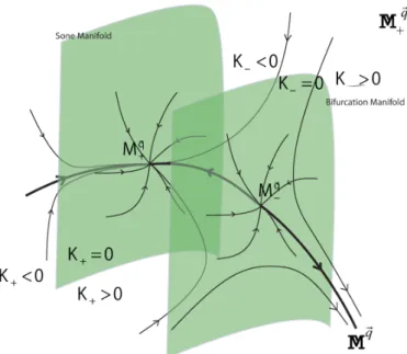
Burgers’ equation (compressiblefluidlike). We illustrate the phase diagram of the

center-stablemanifold of the dynamical system given by (31) around aMaxwellian $M_{0}$ state with

Mach number$=-1.$

The dynamical system on the 1-D invariant

curve

(center manifold) is a Burgers

type ODE (First order ODE). This flow concludes a connecting orbit for the two states

$(M_{-}^{\tilde{q}}, M_{+}^{\vec{q}})$.

This proves the existence of Boltzmann profile as well as the monotone

prop-erty of the profile. This monotone property is a problem raised in [14]. Here, the two

co-dimension 2 invariant submanifolds of the center-stable manifold define two scalar

functions $K$-and $K_{+}$ on the center-stable manifold so that the function $K_{-}$ gives the

bifurcation of the dynamical system; and the function $K_{+}$ defines the hydrodynamics

flows patterns, either a slowly expanded pattern for flows in the region $K_{+}<0$ or an

exponentially fast compressive wave pattern in the region $\{K_{+}>0\}\cup\{K_{-}<0\}$. With

these two functions, one can return to the bifurcation of the Milne’s problem (31). By

Lemma 20 in [20], there is a local 1-1 continuous map $\iota_{\vec{q}}$ from the center-stable manifold

with given macroscopic flux $\vec{q}$ to the space

$L_{\xi,3,+}^{\infty}$, which is the space for the imposed

boundary data. Thus, the sign of the function $K_{-}(\iota_{\vec{q}}(b))$ gives the bifurcation of the

Milne’s problem around the Mach number $=-1$. When Mach number is around $0$, the

$K_{+}$

Figure 1: Two-scale dynamics

on

thecenter-stablemanifold$\mathbb{M}_{+}^{\vec{q}}$ which is the center-stable

manifold with macroscopic flux $\vec{q}\equiv P_{0}\xi^{1}M_{-}.$

4.4

Linear

and nonlinear

wave

scattering around

a

Boltzmann

shock

layer

In[39],

one

considers the Boltzmannequationaround

a

Boltzmannshock profile, $\varphi(x-st)$:

$\{\begin{array}{l}(\partial_{t}-s\partial_{x}F)+\xi^{1}\partial_{x}F-L_{\varphi}F=Q(F) ,F(x, 0)=F_{0}(x) , (posed initial data,)\end{array}$ (41)

where $L_{\varphi}$ is

a

linear collision operator around the shock profile $\varphi$. Suppose that the

Boltzmann shockprofile $\varphi$ is for

a

weak 3-shock

wave

$(\vec{u}_{-},\vec{u}_{+})$ for

a

compressible Euler

equation

as a

system of hyperbolic conservation laws:

$\vec{u}_{t}+\vec{F}(\vec{u})_{x}=0, \vec{u}\in \mathbb{R}^{3}.$

One wants to

remove

the

zero

total macroscopic

mass

condition in [14],

$\int_{R}P_{0}F_{0}(x, 0)dx=0$ (42)

for the purpose to investigate the hydrodynamic limits problem for the Boltzmann

equa-tion, [9, 10].

The main point ison obtaining the optimal linearwave propagationaroundthe

Boltz-mann shock layer and to

use

it to establish the nonlinear

wave

coupling. The central idea

around a shock profile is called the T-C scheme (transverse-compressible scheme). This

scheme is closely related to the Lax’s entropy condition for a p-th shock wave and the

diffusewavesintroduced in [12] to determine the viscous shock profile phase shift. In [39]

one uses the Green’s functions at two far fields to construct

an

approximated solution

$A_{0}(x, t)$ and a local wave front $l_{0}(t)\varphi’(x)$ to approximate the solution of the linearized problem

$(\partial_{t}+(\xi^{1}-s)\partial_{x}-L_{\varphi})f=0$ (43)

to yield that $\mathscr{E}_{0}$, the truncation

error

for (43),

$\mathscr{E}_{0}\equiv(\partial_{t}+(\xi^{1}-s)\partial_{x}-L_{\varphi})(A_{0}(x, t)+l_{0}(t)\varphi’(x))$ (44)

satisfies that following property:

$\{\begin{array}{l}\int_{\pi}(D_{i}, \mathscr{E}_{0}(x, t))dx=0, i=1, 2,\Vert P_{0}\mathscr{E}_{0}(x, t)\Vert_{L_{\xi,3}^{\infty}}\leq O(1)\frac{\epsilon^{2}}{t}e^{-(\epsilon|x|+\epsilon^{2}t)/C_{0}} for t\geq\epsilon^{-2},\Vert P_{1}\mathscr{E}_{0}(x, t)\Vert_{L_{\xi_{1}3}^{\infty}}\leq O(1)\frac{\epsilon}{\sqrt{t}}e^{-(\epsilon|x|+\epsilon^{2}t)/C_{0}} for t\geq\epsilon^{-2},\end{array}$ (45)

where $\epsilon\equiv\Vert\vec{u}_{-}-\vec{u}_{+}\Vert$ and _{$\{D_{1}, D_{2}, M_{-}-M_{+}\}$}

are

the macroscopic dual vectors of

$\{r_{1}(\vec{u}_{-}), r_{2}(\vec{u}_{-}), \vec{u}_{-}-\vec{u}_{+}\}$, and $r_{j}(\vec{u}_{-})$ are the j-th left eigenvectors of $\vec{F}’(\vec{u}_{-})$. The

approximated solution $A_{0}+l_{0}\varphi’$ for (43) with the property (45) is the $T$ part of the T-C

scheme.

Next, one needs to have an exponentially sharpestimate of the output $w(x, t)$ _{due to}

the truncation error $\mathscr{E}(x, t)$:

$\{\begin{array}{l}(\partial_{t}+(\xi^{1}-s)\partial_{x}-L_{\varphi})w=-\mathscr{E}_{0},\int_{\mathbb{R}}P_{0}w(x, 0)dx=0.\end{array}$ (46)

This is a system of equations and there is no spectrum gap property to

assure

an

ex-ponential decayingstructure though $w(O, t)$ will exponentiallyconverge in time. For the

purpose to assert an exponential estimate, oneintroduced adamping to the system (46):

$\{\begin{array}{l}(\partial_{t}+(\xi^{1}-s)\partial_{x}-L_{\varphi})W_{0}=-\mathscr{E}_{0}-\gamma\sum_{j=1}(D_{j}, W_{0})D_{j},\int_{\pi}P_{0}W_{0}(x, 0)dx=0,\end{array}$ (47)

with a small$\gamma>0$. This system possesses conservation laws:

so

that with $\gamma>0$, (48), and

energy

estimates

one

shows that this system will decay in

time exponentially.

Since the truncation

error

$P_{0}\mathscr{E}_{0}$ doesnot

possess

anytransient components, the

damp-ing $- \gamma\sum_{j=1}(D_{j}, W_{0})D_{j}$ is essentiallyvirtual. Hence, the solution $W_{0}(x, t)$ gives

an

expo-nentially sharp approximation to the solution $w_{0}(x, t)$ around _$x=$ O. The construction

of the approximated solution $W_{0}(x, t)$ is called the $C$-part of the T-C scheme. This part

creates another truncation

error

$- \gamma\sum_{l=1}^{2}(D_{l}, W_{0})D_{l}$. Then, this leads to consider the

problem

$\{\begin{array}{l}(\partial_{t}+(\xi^{1}-s)\partial_{x}-L_{\varphi})f_{1}=\gamma\sum_{l=1}^{2}(D_{l}, W_{0})D_{l)}f_{1}(x, 0)=0.\end{array}$ (49)

One repeats the same procedure to give the T-C iteration:

To find $A_{i}$ and $l_{i}(t)$ satisfying

$\{\begin{array}{l}\mathscr{E}_{i}(x, t)\equiv(\partial_{t}+(\xi^{1}-s)\partial_{x}-L_{\varphi})(A_{i}+l_{i}(t)\varphi’)-\gamma\sum_{l=1}^{2}(D_{l}, W_{i-1})D_{l},(\partial_{t}+(\xi^{1}-s)\partial_{x}-L_{\varphi})W_{i}=-\mathscr{E}_{i}-\gamma\sum_{j=1}(D_{j}, W_{i})D_{j},W_{i}(x, 0)=0,\end{array}$ (50)

and the property (45) for $\mathscr{E}_{0}$ still holds for $\mathscr{E}_{i}$. Finally,

one

obtained sharp linear

wave

scattering structure around theshock profile. The linearwave scattering structureis used

to show the pointwise structure of solution of (41)

as

illustrated:

This T-C scheme also works for viscousconservation law. Especially, the sharp

point-wise structure gives advantages in the study of the

case

with presence of boundary in

4.5

Riemann

problem

for shock

wave

data

In [40], one considers the initial value problem (41) with a shock wave initial data $F_{0}(x)$:

$F_{0}(x)=\{\begin{array}{l}M_{\vec{u}-} for x<0,M_{\vec{u}_{+}} for x>0.\end{array}$ (51)

Here, $(\vec{u}_{-},\vec{u}_{+})$ is

a

shock

wave

and $M_{\vec{u}\pm}$

are

Maxwellians related to the states $\vec{u}\pm$; and

$\Vert\vec{u}_{-}-\vec{u}_{+}\Vert=\epsilon\ll 1.$

This problem is a multi-time scale problem. There are five time scales illustrated by the table:

In the time scale

$0<t<1$

, the particlelike structure $\mathbb{P}$

of the Green’s function and

the shock wave initial data force the solution $F(x, t)$ to behave close to the hyperbolic

scale function $f(x/t)$. In the time scale $t\sim 1$, one breaks the collisionoperator into gain

and loss to yield the $O(1)$ structure. When $t\in(1, \epsilon^{-2})$, one

can

linearize the problem at

the Maxwellian $M_{\vec{u}-}$ or$M_{\vec{u}+}$, then by the structure (24)

one

concludes that the structures

resemble to the convected heat equation with speeds $\lambda_{j}$. When $t\in(\epsilon^{-2}, \epsilon^{-2}\log\epsilon)$, one

restricts the macroscopic state on the line segment connecting $M_{\vec{u}-}$ and $M_{\vec{u}+}$ to form an

approximated solution. This restriction carries the spirit of the Chapman-Enskog

expan-sion. One can derive a nonlinear scalar equation close to the viscous Burgers equation.

One can use the Hopf-Cole transform effectivelyto realize the formation of the nonlinear

layer. When $t\sim\epsilon^{-2}\log\epsilon$, one can

use

the formed profile by the Burgers-like equation

and compare it with the Boltzmann shock profile so that one applies the stability of a

shock profile in [40] to yield the global structure of the Riemann problem with a shock

4.6

Future developments

The works done in [4, 15, 19, 20, 39, 40]

are

for planar

wave

motions ofthe Boltzmann

equation. When the perturbations are multi-D, the mathematical analysis of the related

problems are completely open. Indeed, there are many open problems in physics

men-tionedin the classicalbook [35].

About the Boltzmann equation in multi-D, the work in [17] gavethe Green’s function

in

3-D

spacedomain; and

gave a

wave

structure related to Huygen’s principle for the 3-D

d’Alembert

wave

equation. In this aspect, it is interesting to consider the shock profile

stability under a 3-D perturbations and in particular the multi-D hyperbolic scale waves

interact with the viscous shock front. It is also interesting to consider the Riemann

prob-lem without assuming the shock

wave

data. The thermal transpiration flow derivedin[35]

is an interesting physical phenomenon to distinguish the difference between Boltzmann

equation and conventional fluid mechanics. To investigate the geometric effects due to a

physical boundary andto relate it with the geometric theory of diffractions would be very

interesting

as

well.

It is also very interesting to complete the $Grad$_{’s and Sone’s} program _{to study the}

interactions ofthe singular layers (shock layer, initial layer, and boundary layer) for 1-D

problem.

References

[1] Caflisch, R. E.; Nicolaenko, B., Shock profile solutions

_of

the Boltzmann equation,

Comm. Math. Phys., 89 (1982),

161-194.

[2] Carleman, T. Sur LaTh\’eoriede

l’\’Equation

Int\’egrodiff\’erentiellede Boltzmann. Acta

Mathematica 60 (1933), 91-142.

[3] Carleman, T. Probl\’emes math\’ematiques dans la th\’eorie cin\’etique des gaz. (French)

Publ. Sci. Inst. Mittag-Leffler. 2 Almqvist

&

Wiksells Boktryckeri Ab, Uppsala

1957

[4] Deng, Shijin; Wang, Weike; Yu,Shih-Hsien Pointwise convergence toKnudsen layers

of

the Boltzmann equation. Comm. Math. Phys. 281 (2008), no. 2, 287-347

[5] Deng, Shijin; Wang, Weike; Yu, Shih-Hsien, Viscous conservation laws with boundary.

SIAM J. Math. Anal. 44 (2012),

no.

4, 2695-2755

[6] Ellis, R.; Pinsky, M. The first and second fluid approximations to the linearized

Boltzmann equation. J. Math. Pures Appl. 54 (1975), no. 9, 125-156.

[7] Goodman, J. Nonlinear asymptotic stability

_of

viscous shock profiles

_for

conservation

[8] Grad, H. Asymptotic theory

_of

the Boltzmann equation, Physics of Fluids, No. 2 Vol. 6, (1963), 147-181.

[9] Grad, H. $A\mathcal{S}$

ymptotic equivalence

_of

theNavier-Stokes andnonlinear Boltzmann

equa-tions, Proc. Symp. Appl. Math. 17(ed. R.Finn), 154-183, AMS, Providence,

1965.

[10] Grad, H. Proc. Symp. in Appl. Math. 17,

154-183

(1965), Rarified Gas Dynamics, I,

26-59 (1963).

[11] S. Kawashima, A. Matsumura,

&

T. Nishida, On the fluid-dynamicalapproximation

to the Boltzmann equation at the level

_of

the Navier-Stokes equation. Comm. Math.

Phys.

70

(1979),

no.

2,

97-124.

[12] Liu, Tai-Ping, Shock waves and

_diffusion

waves. Nonlinear systems of partial

differ-ential equations in applied mathematics, Part 1 (Santa Fe, N.M., 1984), 283–291,

Lectures in Appl. Math., 23, Amer. Math. Soc., Providence, RI,

1986

[13] Liu, T.-P. Pointwise convergence to shock

waves

_for

viscous conservation laws.

Comm. Pure Appl. Math. 50 (1997), no. 11,

1113–1182.

[14] Liu, T.-P.; Yu, S.-H. Boltzmann Equation: Micro-Macro Decompositions and

Posi-tivity

_of

Shock Profiles, Comm. Math. Phys. 246 (2004), 133-179.

[15] Liu, T.-P.; Yu, S.-H. The Green’s

_function

and large-time behavior

_of

solutions

_for

one-dimensional Boltzmann equation, Comm. Pure. Appl. Math., 57 (2004), no.12,

1543-1608.

[16] Liu, Tai-Ping; Yang, Tong; Yu, Shih-Hsien Energy method

_for

Boltzmann equation.

Phys. D188 (2004),

no.

3-4,

178–192.

[17] Liu, T.-P.; Yu, S.-H. Green’s

_{function of}

Boltzmann equation, 3-D waves, Bull. Inst.

Math. Acad. Sin. (N.S.) 1 (2006), no. 1, 1-78.

[18] Liu, Tai-Ping; Yang, Tong; Yu, Shih-Hsien; Zhao, Hui-Jiang Nonlinear stability

_of

rarefaction

waves

_for

the Boltzmann equation. Arch. Ration. Mech. Anal. 181 (2006),

no. 2, 333–371.

[19] Liu, T.-P.; Yu, S.-H., Initial-bouniary value problem

_for

one-iimensional wave

solu-tions

_of

the Boltzmann equation, Comm. Pure Appl. Math., 60 (2007), no. 3, 295-356.

[20] Liu, T.-P.; Yu, S.-H. Invariant

_{Manifolds for}

steady Boltzmann

_flows

and its

[21] T. Nishida, Takaaki Fluid Fluid dynamical limit

_of

the nonlinear Boltzmann equation

to the level

_of

the compressible Euler equation. Comm. Math. Phys. 61 (1978), no.

2, 119-148

[22] Sone, Y., Kinetic theory analysis of linearized Rayleigh problem, J. Phys. Soc. Jpn

19

(1964),

1463-1473.

[23] Sone, Y., Effect of sudden change of wall temperature in ararefied gas, J. Phys. Soc.

Jpn20 (1965),

222-229.

[24] Sone, Y., Thermalcreep in rarefied gas, J. Phys. Soc. Jpn21 (1966),

1836-1837.

[25] Sone, Y.,Asymptotic theory of flow ofrarefied gas

over

asmooth boundary I, in: L.

Trilling and H. Y. Wachman, eds.,

_Rarefied

Gas Dynamics (Academic Press, New

York), Vol. I, (1969), 243-253.

[26] Sone, Y., Asymptotic theoryofflow ofrarefied gas

over

asmooth boundary II, in: D.

Dini, ed.,

_Rarefied

Gas Dynamics (EditriceTecnico Scientifica, Pisa), Vol. II, (1971),

737-749.

[27] Sone, Y., Kinetic theory of evaporation and condensation Linear and nonlinear

prob-lems, J. Phys. Soc. Jpn45 (1978),

315-320.

[28] Sone, Y., Kinetic theoretical studies of the half-space problem of evaporation and

condensation, Transp. Theory Stat. Phys. 29 (2000),

227-260.

$[29_{\backslash }]$ Sone,Y.; Onishi, Y., Kinetictheory ofevaporation and condensation: Hydrodynamic

equation and slip boundarycondition, J. Phys. Soc. $Jpn44$ (1978), 1981-1994

[30] Sone, Y.; Aoki, $K$; Yamashita, K., A study of unsteady strong condensation

on a

plane condensed phase with special interest in formation of steady profile, in: V.

Boffi and C. Cercignani, eds.,

_Rarefied

Gas Dynamics (Teubner, Stuttgart), Vol. II,

(1986),

323-333.

[31] Sone, Y.; Golse, F.; Ohwada, T.; Doi, T., Analytical study of transonic flows of a

gascondensing onto itsplane condensed phaseonthe basis of kinetic theory, $Eur.$ $J.$

Mech. B/Fluids 17 (1998), 277-306.

[32] Sone, Y., Kinetic theory

_of

evaporation and condensation Linear and nonlinear

prob-lems, J. Phys. Soc. Jpn, 45 (1978), 315-320.

[33] Sone, Y.; Aoki, $K$; Yamashita, K. $\mathcal{A}$

study

_of

unsteady strong condensation

on a

and C. Cercignani,eds., RarefiedGasDynamics(Teubner, Stuttgart),Vol. II, (1986),

323-333.

[34] Sone, Y.; Golse, F.; Ohwada, T.; Doi, T. Analytical study

_of

transonic

_{flows of}

a

gas condensing onto its plane condensedphase on the basis

_of

kinetic theory, Eur. J.

Mech. B/Fluids, 17 (1998), 277-306.

[35] Sone, Y. Molecular Gas Dynamics: Theory, Techniques, and Applications,

Birkhauser, 2007.

[36] Ukai, S. On the existence of global solutions of mixed problem for non-linear

Boltz-mann equation. Proc. Japan Acad. 50 (1974),

179-184.

[37] Ukai, S.; Yang, T.;Yu, S.-H. Nonlinear Boundary Layers of the Boltzmann Equation:

I. Existence. Commun. Math. Phys. 236 (2003),

373-393.

[38] Ukai, S.; Yang, T.; Yu, S.-H. Nonlinear stability

_of

boundary layers

_of

the Boltzmann

equation. I. The case $M \infty\int-1$. Comm. Math. Phys. 244 (2004), no. 1, 99–109.

[39] Yu, Shih-Hsien, Nonlinear wave propagations over a Boltzmann shock profile. J.

Amer. Math. Soc. 23 (2010), no. 4,

1041–1118.

[40] Yu, Shih-Hsien, Initial and Shock Layers

_for

Boltzmann Equation, Arch. Ration.