可積分系によるニューラルネットワークの学習の解析 (離散可積分系の応用数理)

可積分系によるニューラルネットワークの学習の解析

Learning

in

neural

networks

and

an

integrable system

福水健次

理化学研究所

KenjiFukumizu

TheInstitute of Physical and Chemical Research (RIKEN)

$\mathrm{E}$-mail: [email protected]

Abstract

This paper investigates the dynamics of batch learning ofmultilayer neural

net-works inthe asymptoticcase where thenumber of training datais much larger than

the number of parameters. First, wepresent experimental resultson the behavior in

the steepest descent learningofmultilayer perceptrons and three-layer linear neural

networks. We see in these results that strong overtraining, which is the increase of generalizationerrorintraining,occursifthemodel hassurplushiddenunits to realize

the target function. Next, to analyzeovertraining from the theoreticalviewpoint, we

analyze the steepestdescent learning equation ofa three-layer linear neural network,

andtheoreticallyshowthatanetworkwithsurplushidden unitspresentsovertraining.

Fromthis theoreticalanalysis, we can seethat overtraining is not afeature observed

in the final stageoflearning, but it occurs in anintermediatetime interval.

1

Introduction

This paper discusses the dynamics of batch learning in neural networks. Multilayer

networks like multilayer perceptrons have been extensively used in many engineering

ap-plications, in hope that their nonlinear structure inspired by biological neural networks

shows a variety of advantages. However, nonlinearity

causes

weaknesses also. For the

training of

a

neural network, for example, a numerical optimization method like the

er-ror back-propagation (Rumelhart et al., 1986) must be used to find the optimal weight

and bias parameters. It is very important from the practical and theoretical viewpoints

to elucidate the dynamical behavior ofa network in training. Especially, the empirical

error, the objective function ofminimization, and the generalization error, the difference

between the target function and its estimate, are of much interest in many researches.

However, the property of such learning rules have not been clarified completely because of its complex nonlinearity.

In this paper, we focus on overtraining (Amari, 1996) as a typical behavior of learning

in multilayer networks. Overtraining is the increase of the generalization

error

after

some

数理解析研究所講究録

IIIUU$\langle$$\mathrm{U}\mathrm{U}\mathrm{l}1\ovalbox{\tt\small REJECT} 1$ UI 1R1$a$UUII$J$

Figure 1: Overtraining in batchlearning. The empiricalerrordecreases during iterative training,

while the generalization increases aftersome time point.

time point in learning (Fig.1). Although the empirical error is a decreasing function

in principle, it does not

ensure

the decrease of the generalization error defined by only

finite number of training examples. Overtraining is not only oftheoretical interest but of

practical importance, because we should

use

an early stopping technique if overtraining

really exists.

There has been a controversy about the existence of overtraining. Some practitioners

assert that overtraining often happens and propose early stopping methods. Amari et

al. (1996) analyze overtraining theoretically and conclude that the effect of overtraining

is much smaller than what is believed by practitioners. Their analysis is true if the

parameter approaches totheglobal minimum of the empiricalerrorfollowing the statistical

asymptotic theory (Crame’r, 1946). However, the usual asymptotic theory cannot be

applied in overrealizable cases, where the model has surplus hidden units to realize the

target function (Fukumizu, 1996; Fbkumizu, 1997). Possibility ofan overrealizable target

is acommonproperty ofmultilayer models, and theexistence of overtraining in suchcases

has still been anopen problem.

There have been other studies related to overtraining. Baldi and Chauvin (Baldi

&

Chauvin, 1991) theoretically analyze the generalization error of two-layer linear networks

estimating the identity function from noisy data. Although they show overtraining

phe-nomena

under several assumptions, their analysis is very limited in that the overtraining

canbeobservedonlywhen the variance ofthenoise inthe trainingsampleis different from

that of the validation sample. In researches from the viewpoint of statistical mechanics,

overtraining is sometimes used for a different meaning. They observe the increase of the

of parameters, and call it overtraining.

The main purpose of this paper is to discuss overtraining of multilayer networks in

connection with overrealizability. We investigate two models: oneis multilayer perceptrons

with the sigmoidal activation function, and the other is linear neural networks, which we

introduce for the simplicityof analysis. Through experimental results of these models, we

can

conjecture that overtraining

occurs

for overrealizable targets. We theoretically verify

this conjecture in linear neural networks.

This paper is organized

as

follows. Section II gives basic definitions and terminology.

Section III shows experimental results concerning overtraining of multilayer perceptrons

and linear neural networks. In Section IV,

we

theoretically show the existence of

over-training in overrealizable cases oflinear neural networks. Section V includes concluding

remarks.

2

Preliminaries

2.1 Framework

of statistical

learning

In this section, wepresent basic definitions and terminologies used in thispaper. A

feed-forward neural network model

can

be defined by a parametric family of maps $\{f(x;\theta)\}$

from $\mathbb{R}^{L}$

to $\mathbb{R}^{M}$, where

$x$ is

an

inputvector and 9 is a parametervector. The three-layer

network model with $H$ hidden units is defined by

$f^{i}(_{X;} \theta)=j=1\sum Hw_{ij\varphi}(_{k=1}\sum^{L}u_{jkk}x+\zeta_{j})+\eta_{i}$, $(1\leq i\leq M)$ (1)

where $\theta=$ $(w_{11}, \ldots, w_{MH}, \eta_{1}, \ldots , \eta_{M}, u_{11}, \ldots, u_{HL}, \zeta_{1}, \ldots , \zeta_{H})$, and an activation

func-tion$\varphi(t)$ is afunction from$\mathbb{R}$to $\mathbb{R}$. We call athree-layer network a multilayerperceptron,

ifthe sigmoidal function

$\varphi(t)=\frac{1}{1+e^{-t}}$ (2)

is used for the activation function.

We use such a model for regression problems, assuming that

an

output of the target

system is observed with a measurement noise. A sample $(x, y)$ from the target system

satisfies

$y=f(X)+v$ , (3)

where$f(x)$ isthe target

function

whichisunknown to alearner, and$v$ is arandom vector

with $0$ as its mean and $\sigma^{2}I_{M}$ as its variance-covariance matrix. We write $I_{M}$ for the

$M\cross M$ unit matrix. An input vector $x$ is generated randomly with its probability density

function $q(x)$, which is unknown to

a

learner. ’baining data $\{(x^{(\nu)}, y)(\nu)|\mathcal{U}=1, \ldots , N\}$

are independent samplesfrom the joint distributionof$q(x)$ and $\mathrm{e}\mathrm{q}.(3)$

.

The parameter 9

is estimated based on the training data without knowing $f(x)$ so _{that a neural network}

can

give

a

good estimate of the target function $f(x)$.

We discuss the least square

error

(LSE) estimator. The objective of training is to find

the parameter that minimizes the following empirical error:

$\mathrm{E}_{emp}(\theta)\equiv\sum_{\nu=1}||yNf(\nu)-(X(\nu)\theta);||^{2}$

.

(4)

Generally, it is very difficult to solve the LSE estimator analytically if the model is

non-linear. Some numerical optimization method is needed to obtain an approximation. One

widely-usedmethodis the steepest descent method, which iteratively updates the

param-eter vector 9 in the steepestdescent direction ofthe error surface definedby $\mathrm{E}_{emp}(\theta)$. The

learning rule is given by

$\theta(t+1)=\theta(t)-\beta\frac{\partial \mathrm{E}_{emp}(\mathit{9}(t))}{\partial\theta}$, (5)

where $\beta>0$is alearning constant. Inthis paper, we discuss only batch learning, inwhich

we calculate thegradient usingall thetraining data. There are manyresearches on online

learning, in which the parameter is always updated for a newlygenerated data (Heskes&

Kappen, 1991).

The performance of a network is often evaluated by the generalization error, which

represents the average

error

between the target function and its estimate. Moreprecisely,

it is defined by

$\mathrm{E}_{gen}(\mathit{9})\equiv\int||f(x;\theta)-f(x)||2q(x)dX$

.

(6)

It is easy to see

$\int\int||y-f(X;\mathit{9})||2p(y|X)q(X)dydx=M\sigma^{2}+\mathrm{E}_{gen}$, (7)

where$p(y|x)$ is the densityfunction of the conditional probability of$y$ given $x$

.

Sincethe

empirical error divided by $N$ approaches to the left hand side of $\mathrm{e}\mathrm{q}.(7)$ when $N$ goes to

infinity, the rninimization of the empiricalerrorroughly approximates the minimizationof

the generalization error. However, they are not exactly the same, and the decrease of the

empiricalerrorduring learning does not ensurethe decrease of the generalization error. It

is extremely important to elucidate the dynamical behavior of the generalizationerror. A

curve

showing the $\mathrm{e}\mathrm{m}\mathrm{p}\mathrm{i}\mathrm{r}\mathrm{i}\mathrm{c}\mathrm{a}\mathrm{l}/\mathrm{g}\mathrm{e}\mathrm{n}\mathrm{e}\mathrm{r}\mathrm{a}\mathrm{l}\mathrm{i}\mathrm{z}\mathrm{a}\mathrm{t}\mathrm{i}\mathrm{o}\mathrm{n}$error as a function oftime is called a learning

Target _Model

Figure 2: Illustration ofan overrealizable case.

In our theoretical discussion, we consider the

case

where $f(x)$ is perfectly realized by

the prepared model; that is, there is a true parameter $\theta_{0}$ such that $f(x;\mathit{9}0)=f(x)$

.

Assume that the model has $H$ hidden units. If the target function $f(x)$ is realized by

a network with a smaller number of hidden units than $H$, we call it overrealizable (see

Fig.2). Otherwise, we call it regular. We focus on the difference of dynamical behaviors

between these two cases.

2.2

Linear

neural networks

We introduce the three-layer linear neural network model

as

the simplest multilayer

modelwhose theoretical analysis is possible. We must be very careful in discussing

exper-imentalresults onlearning ofa multilayer perceptron especially inan overrealizable case.

In such a case, around the global minimum there exists a high-dimensional subvariety on

which $\mathrm{E}_{emp}$ is very close to the minimum (Fukumizu, 1997). The convergence oflearning

is much slower than the convergence in regular

cases

because the gradient is very small

aroundthis subvariety. In addition, of course, learning with

a

gradient methodsuffers from

local minima, which is a common problem to all nonlinear models. We cannot exclude

their effects, and this often makes derived conclusions obscure. On the other hand, the

theoreticalanalysis oflinear neural networks ispossible (Baldi&Hornik, 1995; Fukumizu,

1997), and the dynamical behavior of the generalization

error

is analyzed in Section 4.

A linear neural network has the identity function for the activation function. In this

paper, we do notusethebiasterms $\eta$and $\zeta$ in linear neural networksforsimplicity. Thus,

a linear neural network is defined by

$f(x;A, B)=BAx$ , (8)

where $A$ is a $H\cross L$ matrix and $B$ is a $M\cross H$ matrix. We assume $H\leq L$ and $H\leq M$

throughout this paper. Although the function $f(x;A, B)$ is linear, $\mathrm{h}\mathrm{o}\mathrm{m}$ the assumption

on

$H$, the model is not equal to the set of all the linear maps from $\mathbb{R}^{L}$

to $\mathbb{R}^{M}$, but is the

set ofthe linear maps of rank no greater than $H$

.

Then, it is not equivalent to the usual

linear regression model $f(x;c)=Cx$ ($C$

:

$M\mathrm{x}L$ matrix). In this sense, the three-layer

linear neural network model is the simplest multilayer model.

3

Learning

curves–experimental

study-In this section, we experimentally investigate the generalizationerror ofmultilayer

per-ceptrons and linear neural networks to

see

their actual behaviors, emphasizing on

over-training.

The steepest descent method $(\mathrm{e}\mathrm{q}.(5))$ in multilayer perceptron leads the well-known

error back-propagation rule (Rumelhart, 1986), which is given by

$w_{ij}(t+1)$ $=$ $w_{ij}(t)+ \beta\sum_{\nu}N=1i\delta^{(\nu)}(t)s_{j}^{(}(\nu)t)$,

$\eta_{i}(t+1)$ $=$ $\eta_{i}(t)+\beta\sum^{N}\nu=1\delta^{()}i\nu(t)$,

$u_{jk()}t+1$ $=$ $u_{jk}(t)+ \beta\sum^{N}\nu=1^{\sum w_{ij}\delta_{i}}i=M1(\nu)(t)_{S_{j}}(\nu)(t)(1-S(\nu)(jt))Xk(\nu)$,

$\zeta_{j}(t+1)$ $=$ $\zeta_{j(t)+\beta\sum\sum_{i1}}\nu=N1M=wij\delta_{i}(\nu)(t)_{S_{j}}(\nu)(t)(1-s_{j}(\nu)(t))$, (9)

where

$\delta_{i}^{(\nu)}(t)=yi(\nu)-f_{i}(X)(\nu;\mathit{9}(t))$, $s_{j}^{(\nu)}(t)=s( \sum_{k=1}^{L(}u_{j}k(t)X_{k}+\zeta j(\nu)t))$ . (10)

Toavoid the problems discussedinSection2.2 asmuchas possible,we adoptthe following

configuration in our experiments. Themodel in usehas 1 input unit, 2 hidden units, and

1 output unit. For a fixed set of training examples, 30 different values are tried for an

initial parameter vector. We select the trial that gives the leastempiricalerrorafter500000

iterations. Figure3 shows theaverage ofgeneralizationerrors over 30different simulations

changing the set of trainingdata. It shows clear overtraining in the overrealizable

case.

On

the other hand, the learning curve in the regular

case

shows no meaningful overtraining.

It isknownthat the LSE estimator of the linear neural network model can be analytically

solvable (Baldi&Hornik, 1995). Although it is practically absurd, of course, to use the

steepest descent method, our interest is not only the optimal estimator but the dynamics

Figure 3: Average learning curves of MLP. The input samples are independent samples from

$N(\mathrm{O}, 4)$, and the output samples include the observation noise subject to $N(\mathrm{O}, 10^{-4})$. The total

number oftraining data is 100. The constant zero function is used for the overrealizable target

function, and$f(x)=s(x+1)+s(x-1)$ is usedfor theregular target. The dottedline shows the

theoretical expectation ofthegeneralizationerror ofthe LSEestimator when the target function

is regularand the usual asymptotic theory is applicable.

here. For the training data of

a

linear neural network, we use the notations;

$X=$

, $\mathrm{Y}=$ . (11)

The empirical

error can

bewritten by

$\mathrm{E}_{emp}=\mathrm{b}[(\mathrm{Y}-xA\tau B^{\tau})T(Y-XATB\tau)]$. (12)

The learning rule ofa linear neural network is given by

$\{$

$A(t+1)$ $=A(t)+\beta\{B^{T}Y^{\tau\tau}X-BBAX^{\tau}X\}$,

$B(t+1)$ $=B(t)+\beta\{\mathrm{Y}\tau XAT-BAx\tau xAT\}$

.

(13)

It is also known that all the critical points but the global minimum of $\mathrm{E}_{emp}$ are saddle

points (Baldi&Hornik, 1995). Therefore, ifwe theoretically consider

a

continuous-time

learning equation, it converges to the global minimum for almost all initial conditions.

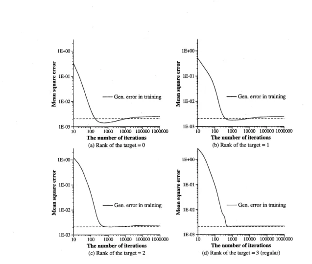
Figure 4 shows the average of learning

curves

for 100 simulations with various training

data from the

same

probability. The number of input units, hidden units, and output

units of the model are 5, 3, and 5 respectively. All the overrealizable cases show clear

overtraining. while the regular case does not show meaningful overtraining. We can also

see that overtraining is stronger when the rank of the target is smaller.

Figure4: Averagelearningcurvesoflinearneural networks. The input samplesareindependent

samplesfrom$N(0, I_{5})$, and the output samples includethe observation noisesubject to$N(0,10^{-2})$.

Thetotal numberoftrainingdatais 100. The dottedline shows the theoretical expectation ofthe

generalizationerrorof theLSEestimator for the regular target.

From these results, we can conjecture that there isan essential difference in the

dynam-ics of learning between regular and overrealizable cases, and overtraining is a universal

property of the latter

cases.

If

we use

a good stopping criterion, the multilayer networks

may have an advantage over conventional linear models, in that the degrade of the

gen-eralization errorby redundant parameters is not socritical as conventional linear models.

Such overtraining in overrealizable

cases

has not been explained theoretically yet. In the

next section,

we

theoretically verify the result in linear neural networks by obtaining the

4

Solvable

dynamics of learning

in linear

neural networks

To verify the existence of overtraining in linear neural networks,weanalyzethe

continuous-time differential equation instead of the discrete-continuous-time learning rule. Although the behavior

ofthe continuousoneand thediscrete

one are

not identical, they showverysimilar

qualita-tive behaviors in computer simulations. We further approximate the differential equation

to derive a solvable

one.

This approximation alsoaffects the solution quantitatively.

How-ever, we can

see

in experiments that similar the original one and the approximated

one

show similar properties in their learning curves, and we can show the existence of

over-training in overrealizable cases.

4.1

Solution

_of.

learning dynamics

Inthe rest of the paper,

we

put the following assumptions;

(a) $H\leq L=M$,

(b) $f(x)=B0A0X$,

(c) $\mathrm{E}[xx^{T}]=\tau^{2}I_{L}$,

(d) $A(0)A(0)^{\tau}=B(0)^{\tau_{B(}}\mathrm{o})$,

(e) The rank of$A(\mathrm{O})$ (or, equivalently under (d), the rankof$B(\mathrm{O})$ ) is $H$

.

Under theseassumptions, $A^{T}$ and_$B$ are _{$L\cross H$}matrixes. Theparameterizationofalinear

neural networkhas$H^{2}$ dimensional redundancy by the multiplication of_{$H\cross H$}nonsingular

matrix from the left of$A$ and its inverse from the right of$B$. The initial condition (d)

does not restrict possible initialization, since it reduces this redundancy with $\frac{1}{2}H(H+1)$

restrictions. The assumption (e) is important in the following discussion. If the rank of

$A(\mathrm{O})$ (or $B(\mathrm{O})$) is less than $H$, the final state of the variables changes, while we do not

discuss it in this paper.

If

we

divide the output as

$\mathrm{Y}=XA_{00}^{\tau_{B^{\tau}V}}+$, (14)

the differential equation of the steepest descent learning is given by

$\{$

$\lrcorner\dot{4}$

$=\beta(B\tau B_{0}A_{0}X\tau x+B^{T}V\tau x-B\tau BAX\tau x)$,

$\dot{B}$

$=\beta(B_{00}Ax^{T\tau}xA+V^{T}XA^{\tau}-BAX^{T}XA\tau)$

.

(15)

This is a nonlinear differential equation which has the terms of the third order. Let

$Z_{O}:= \frac{1}{\sigma}V^{\tau}X(XTx)^{-1}/2$

.

It is easy to see that $Z_{O}$ is independent of$X$, and that all the

elements of$Z_{O}$

are

mutually independent and subject to $N(\mathrm{O}, 1)$

.

We decompose$X^{T}X$ as

$X^{T}X=\tau^{2}NI_{L}+\tau^{2\sqrt{N}z_{I}}$, ₍₁₆₎

31

where the off-diagonal elements of$Z_{I}$ aresubject to$N(\mathrm{O}, 1)$ andthe diagonal elements

are

subject to $N(0,2)$ if$N$ goes to infinity. Let

$F=B_{0}A_{0}+ \frac{1}{\sqrt{N}}(B_{0}A_{0}Z_{I}+\frac{\sigma}{\tau}Z_{O})$. (17)

We neglect the order $O(\sqrt{N})$ in the nonlinear terms to derive a solvable equation, and

approximate $\mathrm{e}\mathrm{q}.(15)$ by $\{$ $I\dot{4}$ $=\beta\tau^{2}NBTF-\beta \mathcal{T}2NB^{T}BA$, $\dot{B}$ _{$=\beta\tau^{2\tau}NFA-\beta_{\mathcal{T}N}2BAA^{\tau}$}

.

(18)

$\mathrm{E}\mathrm{q}.(18)$ is a good approximation of the original$\mathrm{e}\mathrm{q}.(15)$ if$N$ is very large.

We further put an assumption:

(f) The rank of$B(0)+FA(0)^{T}$ _is $H$.

This assumption is a technical one, which is used to prove overtraining. The assumption

(f) is almost always satisfied if the initial condition is independent of$F$

.

We have $AA^{T}=B^{T}B$ _{because of the fact} $\frac{d}{dt}(AA^{T})=\frac{d}{dt}(B^{T}B)$ andthe assumption (d).

Ifwe introduce $2L\cross H$ matrix

$R=$

, (19) then, $R$ satisfies the differential equation

$\frac{dR}{dt}=\beta\tau^{2}NSR-\frac{\beta\tau^{2}N}{2}RR^{T}R$, where

$S=$

. (20)

This is very sinilar to Oja’s learning equation (Oja, 1989; Yanet al., 1994), orthe

general-ized Rayleigh quotient (Helmke&Moore, 1994), whichis knownto beasolvable nonlinear

differential equation (Yan et al., 1994).

Thekey fact to solve $\mathrm{e}\mathrm{q}.(20)$ is to derivethe differential equation on $RR^{T}$:

$\frac{d}{dt}(RR^{T})=\beta\tau^{2}NsRR^{\tau}+\beta_{\mathcal{T}^{2}N}RR\tau s-\beta \mathcal{T}^{2T}N(RR)2$

.

(21)

This is

a

matrix Riccati differential equation and well-known to be solvable. We have the

following

Theorem 1. Assume that the rank

_of

$R(\mathrm{O})$ is

full.

Then, the Riccati

differential

equation

(21) has a unique solution

_for

all $t\geq 0$, and the solution is given by

$R(t)R^{T}(t)=e^{\beta\tau^{2}N}Rst( \mathrm{o})[I_{H}+\frac{1}{2}R(\mathrm{o})T\{e^{\beta_{\mathcal{T}^{2}N}t}S-1\beta \mathcal{T}NSt-se-1\}S2R(\mathrm{o})]^{-1}R(0)^{T\beta t}e\tau N2S$

.

(22)

For the proof, see Sasagawa (1982) and Yanet al. (1994). Using this theorem,

we

easily

obtain the following theorem in the

same

manner asYan et al. (1994, Theorem 2.1).

Theorem 2. Assume that the rank

_of

$R(\mathrm{O})$ is

full.

Then, the

differential

equation (20)

has a unique solution

_for

all$t\geq 0$, and the solution is expressed as

$R(t)$ $=$ $e^{\beta_{\mathcal{T}^{2}}NS}tR( \mathrm{o})[I_{H}+\frac{1}{2}R(0)^{\tau}\{e\tau\beta 2Ns_{S^{-}}t1\beta\tau^{2}Nst-se-1\}R(0)]^{-\frac{1}{2}}U(t)$, (23)

where $U(t)$ is a $H\cross H$ orthogonal matrix.

4.2

Dynamical behavior of the generalization

error

In this subsection, we write $M(l\cross n;\mathbb{R})$ for the set of real $l\cross n$ matrixes. Using the

assumption (c), the generalization error is written as

$\mathrm{E}_{gen}=\tau^{2}\mathrm{b}[(BA-B0A_{0})(BA-B0^{A_{0})^{\tau}}]$. (24)

It is easyto see that the derivative of$\mathrm{E}_{gen}$ is

$\frac{d}{dt}\mathrm{E}_{gen}=\beta\tau^{4}N$

{Tr

$[(F-BA)A^{\tau}A(BA-B_{0^{A0}})^{\tau}]+\mathrm{n}[BB^{\tau_{()(}T}F-BABA-B0^{A_{0})}]$

}

(25)

Note that a transform of the input or output vectors by an orthogonal matrix does not

change the generalization error. Therefore, using the singular value decomposition of

$B_{0^{A}0_{)}}$

we

can

assume

without loss of generality that $B_{0}A_{0}$ is diagonal;

$B_{0}A_{0=}$

,

_{$\Lambda^{(0)}=$}

, (26)

where $r$ is the rank of $B_{0}A_{0}$, and $\lambda_{1}^{(0)}\geq\cdots\geq\lambda_{r}^{(0)}>0$ are the singular values of $B_{0}A_{0}$

.

The rank $r$ is equal to or less than $H$

.

The target function is overrealizable ifandonly if $r<H$.

We employ the singular value decomposition of$F$,

$F=W\Lambda U^{T}$

.

(27)

In this equation, $U$ and $W$ are $L$ dimensional orthogonal matrixes, and

$\Lambda=$

, (28)

where $\lambda_{1}\geq\lambda_{2}\geq\cdots\lambda_{L}\geq 0$

are

the singular values of$F$. We

assume

that $\lambda_{1}>\lambda_{2}>\cdots>$

$\lambda_{L}>0$. This is satisfied almost surely because of the stochastic noise in$F$

.

We write, for

simplicity,

$F=B_{0}A_{0}+\mathcal{E}Z$, (29)

where $\epsilon=\frac{1}{\sqrt{N}}$

.

We further put anassumption:

(g) $\lambda_{r}^{(0)}>>\epsilon$and _{$1\gg\epsilon$}

.

The above assumption asserts that the number of data is large enough to discriminate between $\lambda_{r}^{(0)}$

and the stochastic deviation from zero. We say $a$ is of the constant order if

$a>>\epsilon$.

It is known that a small perturbation of a matrix

causes

a perturbation of the same

order to the singular values (see Bartia, 1997, Section III, for example). The diagonal

matrix A is decomposed as

$\Lambda=$

,

(30) where

$\Lambda_{1}==$

, (31)

$\epsilon\tilde{\Lambda}_{2}==$

, (32)

$\epsilon\tilde{\Lambda}_{3}==$ .

(33)

Note that the normalized singular values $\overline{\lambda}_{j}(r+1\leq j\leq L)$

are

of the constant order.

The purpose of this subsection is to show that

$\frac{d}{dt}\mathrm{E}_{gen}>0$ (34)

if$r<H$ (overrealizable) and$t$ satisfies

If this is proved, it

means

the existence of overtraining in overrealizable

cases.

Before

enteringinto the details, we give an intuitive description of what happens in the learning

process ofanetwork (Fukumizu, 1998). The final state of the solution can be written by

$W\Lambda^{\frac{1}{2}}\Lambda^{\frac{1}{2}}U^{T}$

.

(36)

This can be considered as the projection of A to the first $H$ eigenspaces. We can deduce

from $\mathrm{e}\mathrm{q}.(22)$ that the solution isalso approximately considered tobe

a

projection of A to

a

$H$ dimensional subspace, which converges to $I_{H}$ exponentially. An important point is

that the convergence speed of the first $r$ components and the rest are different if$r<H$

.

Theorder of the former is roughly$o(e^{-aNt})$ and the latter is $o(e^{-b\sqrt{N}t})$for

some

constant

$a$ and $b$

.

When the slow dynamics of the latter is the leading factor, the subspace of the

projectionis approximately

$\Pi=(_{0}^{I_{r}}0$ $o(e^{-})I_{Hr)}\mathrm{o}-\sqrt{N}t$ . (37)

It is easy to

see

the shrinkage of the components corresponding to $H-r$ redundant

pa-rameters in the projection$\Lambda^{-\frac{1}{2}}\Pi(\Pi\tau\Pi)-1_{\Pi}\tau_{\Lambda^{-}}\frac{1}{2}$. Thissuppresses theeffect of stochastic

noise and makes a betterestimation than the final one.

Let

us

start the theoretical verification with the singular valuedecompositionsto simplify

$\mathrm{e}\mathrm{q}.(25)$. We have

$S=\Phi\Phi^{T}$ , (38)

where $\Phi=\frac{1}{\sqrt{2}}(_{W-W}^{UU})$

.

From the assumption (d), the singular value decomposition of

$R(\mathrm{O})$ has the following form;

$R(0)=\Theta J\Gamma G^{\tau}$, (39)

where

$\Theta=$

,

$J=$

, and

$\Gamma=$

.

(40)

The matrixes $P,$ $Q$ and $G$ are $L,$ $L$, and $H$ dimensional orthogonal matrixes respectively.

Because of the assumption (e), $\Gamma$ is invertible. Using these decompositions, $RR^{T}$ can be

rewritten as

$RR^{T}=\Phi(e^{\beta\tau_{0}^{2}N}0\Lambda te^{-\beta N\Lambda}\tau^{2}t)\Phi^{T}\Theta J$

$\cross[\Gamma^{-2}+\frac{1}{2}J\tau\ominus\tau_{\Phi\{}-\}\Phi^{T}\ominus J]^{-1}$

$\mathrm{x}J^{T}\ominus T\Phi(e^{\beta\tau_{0}^{2}}0N\Lambda te^{-\beta_{\mathcal{T}N}}2\Lambda t)\Phi^{T}$

.

(41)

Let $C=(U^{T}P+W^{T}Q)$ _and$D=(U^{\tau_{P-W}\tau}Q)$

.

_Decompose these two matrixes as

$C=$

,

$D=$

,

(42)

where $C_{H},$$D_{H}\in M(H\cross H;\mathbb{R})$, and $C_{3},$_{$D_{3}\in M((L-H)\cross H;\mathbb{R})$}

.

Then, we have

$\Phi^{T}\Theta J=\frac{1}{\sqrt{2}}$

, (43)

where$\Lambda_{H}=(_{0}^{\Lambda_{1}}\Lambda_{2}0)$

.

Since$B(0)+FA(0)^{T}=Q(_{\mathit{0}}^{\mathrm{r}})G^{T}+W\Lambda U\tau P(_{\mathit{0}}\Gamma)c^{\tau_{7}}$ the

assump-tion (f)

assures

that $C_{H}$ is invertible. If we introduce

$K=$

(44)

$\mathrm{e}\mathrm{q}.(41)$ canbe rewritten as

$RR^{T}=2\Phi(_{0}^{\Lambda^{\frac{1}{2}}}$ $\sqrt{-1}\Lambda^{\frac{1}{2}\mathrm{I}^{K}\Psi}0-1KT(_{0}^{\Lambda^{\frac{1}{2}}}$ $\sqrt{-1}\Lambda^{\frac{1}{2})}0\Phi^{T}$, (45)

where

$\Psi=K^{\tau_{K+\Lambda}\frac{1}{H2}\beta N\Lambda_{H}}e^{-}\tau 2tC_{H}^{\tau}\Gamma-2CHe-\beta\tau^{2}N\Lambda H{}^{t}\Lambda^{\frac{1}{H2}}$

$+e^{-2\beta_{\mathcal{T}^{2}N}H}+ \Lambda t\Lambda e-\beta \mathcal{T}N2\Lambda_{H}{}^{t}C\frac{1}{H2}-1Tc3\tau\Lambda-1\mathit{0}3C_{H}-1\beta\tau N2\Lambda H{}^{t}\Lambda H3\frac{1}{H2}e^{-}$

$- \Lambda^{\frac{1}{H2}}e-\beta_{\mathcal{T}}2N\Lambda_{H}tC_{H}-1T-1-D^{\tau_{\Lambda D_{H}C_{H}{}^{t}\Lambda}}HH\frac{1}{H2}1-e\beta\tau^{2}N\Lambda H$

Note that $K\Psi^{-1}K^{T}$ is exponentially close to the orthogonal projection onto the subspace

spanned bythe.first $H$ components.

In the matrix $K$, the $(H+1, H)$-component has the slowest order in the convergence,

and the order is $\exp\{-\beta\tau^{2\sqrt{N}-}(\tilde{\lambda}H\tilde{\lambda}H+1)t\}$

.

Hereafter,

we assume

that there is a time

interval such that the value of this component is very small but sufficiently larger than $\epsilon$;

that is,

$\epsilon<<\exp\{-\beta_{\mathcal{T}}2\sqrt{N}(\tilde{\lambda}_{H}-\tilde{\lambda}H+1)t\}<<1$

.

(47)

This is equivalent to the condition of $\mathrm{e}\mathrm{q}.(35)$. We consider the main part of $K\Psi^{-1}K^{T}$,

neglecting terms offaster convergence.

The matrix $K$

can

befurther decomposed

as

$K==$

, (48)

where$K_{21},$$K_{41}\in M((L-H)\cross r;\mathbb{R}),$ $K_{22},$$K_{42}\in M((L-H)\cross(H-r)),$$K_{31}\in M(H\mathrm{x}r;\mathbb{R})$,

and $K_{32}\in M(H\cross(H-r))$. The convergence of$K_{21},$ $K_{3}$, and $K_{41}$ is equal to or faster

than the order of$\exp\{-\beta_{\mathcal{T}N}2(\lambda r-\epsilon\tilde{\lambda}r+1)t\}$. We further assume that

$\exp\{-\beta\tau^{2}N(\lambda r-\epsilon\tilde{\lambda}_{r}+1)t\}<<\epsilon^{\frac{3}{2}}\exp\{-2\beta\tau 2_{\sqrt{N}()t}\tilde{\lambda}_{H}-\tilde{\lambda}H+1\}$ (49)

holds in the interval of$\mathrm{e}\mathrm{q}.(47)$. This assumption is naturally satisfied under the condition

of$\mathrm{e}\mathrm{q}.(35)$ if$N$ is sufficiently large, since it is equivalent to

$t>> \frac{\frac{3}{2}\log^{\sqrt{N}}}{\beta_{\mathcal{T}^{2}N}\{\lambda r+\frac{1}{\sqrt{N}}(\tilde{\lambda}H-\tilde{\lambda}r+1+\tilde{\lambda}_{H+1})\}}$. (50)

Hereafter, we $\mathrm{u}\mathrm{s}\mathrm{e}\sim \mathrm{f}\mathrm{o}\mathrm{r}$ an approximation up to the leading order of each component in

matrixes. Then, the solution can be rewritten as

$RR^{T}$ $2\Phi(_{0}^{\Lambda^{\frac{1}{2}}}$ $\sqrt{-1}\Lambda^{\frac{1}{2})\tau_{K)K^{T}}}0K(I_{H}-K22(_{0}^{\Lambda^{\frac{1}{2}}}$ $\sqrt{-1}\Lambda^{\frac{1}{2})}0\Phi^{T}$

$2\Phi\Phi^{T}$

.

(51)

Therefore, we obtain

$A^{T}.A$ $U\Lambda^{\frac{1}{2}}\Lambda^{\frac{1}{2}}U^{T}$, $BA$ $W\Lambda^{\frac{1}{2}}\Lambda^{\frac{1}{2}}U^{T}$

,

$BB^{T}$ _{$W\Lambda^{\frac{1}{2}}\Lambda^{\frac{1}{2}}W^{T}$}

.

(52)

Now, we are in a position to prove overtraining. The first term in the right hand side of$\mathrm{e}\mathrm{q}.(25)$ is written as

Tr$[(F-BA)A\tau A(BA-B0A\mathrm{o})T]$

$\sim \mathrm{h}[\Lambda^{\frac{1}{2}}\Lambda\Lambda^{\frac{1}{2}}$

$\cross\{\Lambda^{\frac{1}{2}}\Lambda^{\frac{1}{2}}-W^{T}B_{0}A0U\}]$ . (53)

Lemma 1 in Appendix and furtherdecompositionof$K_{2}$ and $K_{4}$ show

Tr$[(F-BA)A\tau A(BA-B_{0}A0)^{\tau}]$

$\sim \mathrm{b}[(_{-\epsilon’\tilde{\Lambda}^{\frac{12}{32}}K_{2}}^{\Lambda^{\frac{1}{\tilde{\Lambda}12}}}\epsilon^{\frac{1}{2}\frac{1}{\underline 2,1\sim 2}}K\tau_{2}K_{2}1\frac{3}{12}K21TK_{21}\Lambda^{\frac{3}{\Lambda 12}}1\Lambda\frac{3}{12}$ $\epsilon^{2}\overline{\Lambda}^{\frac{1}{22}}(KK\tilde{\Lambda}--\epsilon^{2}\tilde{\Lambda}^{\frac{2T1}{\mathrm{s}^{2}}}K\epsilon_{222}^{\frac{3}{2}}\Lambda^{\frac{1}{12}\tau_{12}}22\tilde{\Lambda}^{\frac{32}{22}}+\epsilon^{2}\tilde{\Lambda}^{\frac{3}{\mathrm{s}^{2}}}K2K2\tilde{\Lambda}^{\frac{3}{\tilde{\Lambda}22}}K2\tau K22\tilde{\Lambda}\frac{1}{22}23K22\tilde{\Lambda}^{\frac{)1}{22}} \epsilon^{2}\overline{\Lambda}^{\frac{1}{32}}(-222+K_{22})T\tau\overline{\Lambda}\epsilon^{\frac{3}{2}\Lambda}\epsilon_{K\tilde{\Lambda}_{22}}2\tilde{\Lambda}^{\frac{\frac{1}{112}}{22}}K\tau K_{2}2\tilde{\Lambda}K222K_{2}\tau\tilde{\Lambda}\frac{\frac{1}{212}}{3K2}2\tau_{K\tilde{\Lambda}_{3}}K\tilde{\Lambda}2K2\tau 1222\tilde{\Lambda}222\frac{1}{\mathrm{s}^{2}})$

$\cross(_{\epsilon^{\frac{1}{2}}\tilde{\Lambda}^{\frac{1}{32}}}-\epsilon^{\frac{1}{2}}\overline{\Lambda}^{\frac{1}{22}}K_{222}^{\tau_{2}}K)KO(\epsilon\Lambda\frac{1}{12}+1\Lambda\frac{11}{12}+O(\in)O(\Xi) \epsilon\tilde{\Lambda}_{2^{-\mathcal{E}}}\tilde{\Lambda}\frac{1}{22}K\tau K_{22}-\epsilon^{\frac{1}{2}}\Lambda^{\frac{1}{12}}K\tau_{12}K\Xi\tilde{\Lambda}^{\frac{1}{32}}K_{2}2\tilde{\Lambda}\frac{1}{22}+O^{+}(\epsilon 2)22222\tilde{\Lambda}\frac{1}{\tilde{\Lambda}22}\frac{1}{22}+o_{(}o(\epsilon)\mathcal{E})$ $\epsilon\tilde{\Lambda}^{\frac{1}{32}}K_{2}2K6^{\frac{1}{2}\frac{1}{12}}\epsilon\tilde{\Lambda}\frac{\Lambda 1}{22}KT2K_{2}22\tau\frac{1}{32}\tilde{\Lambda}^{\frac{\tilde{\Lambda 1}}{32}}O(\epsilon)2)_{(54)}1\tau\tilde{\Lambda}\frac{+1}{32}2++o(\Xi O(\in))2]$ .

The leading order is $\epsilon^{3}\exp\{-2\beta\tau\sqrt{N}2(\tilde{\lambda}_{H}-\tilde{\lambda}_{H+1})t\}$. Note that the order $O(\epsilon^{4})\cross$

$\exp\{-\beta_{\mathcal{T}}2\sqrt{N}(\tilde{\lambda}H-\tilde{\lambda}H+1)t\}$, appeared in $(3, 2)$ _{$\cross(2,3)$} part in $\mathrm{e}\mathrm{q}.(54)$, is smaller under

the condition of $\mathrm{e}\mathrm{q}.(47)$, and the order $o(\epsilon^{\frac{3}{2}})\cross K_{21}$, appeared in the $(3, 1)$ $\cross(1,3)$ part,

is also smaller under the assumption of$\mathrm{e}\mathrm{q}.(49)$. Thus, the main part is included in

Tr$[ \epsilon^{3}\tilde{\Lambda}^{\frac{1}{22}}K_{22}\tau K22\tilde{\Lambda}\frac{5}{22}-\mathit{6}3\tilde{\Lambda}^{\frac{1}{22}}K2T\tilde{\Lambda}_{3}2K22\overline{\Lambda}^{\frac{3}{22}}-\epsilon^{32}\tilde{\Lambda}^{\frac{1}{32}}K_{22}\tilde{\Lambda}_{2}K^{\tau_{2}}2\tilde{\Lambda}\frac{1}{32}\in^{3}+\tilde{\Lambda}^{\frac{3}{32}}K22\tilde{\Lambda}2K2\tau_{2}\tilde{\Lambda}\frac{1}{32}]$

$= \in^{3}\sum_{i=1j}^{L-H}\sum_{1=}\overline{\lambda}r+j(\tilde{\lambda}r+i-\tilde{\lambda}H+i)^{2}\mathrm{t}(K_{2}H-r)2ij\}^{2}$

.

(55)

All the terms in $\mathrm{e}\mathrm{q}.(55)$ are positive, and this proves the trace is strictly positive. It

can

Thus, we obtain

$\frac{d}{dt}\mathrm{E}_{gen}>0$ (56)

ifthe target is overrealizable and $t$ is in the interval of$\mathrm{e}\mathrm{q}.(35)$.

From the above discussion,

we

can see

that overtraining occurs in

an

intermediate

in-terval, while overtraining of the

average

learning

curve

in Fig.4

seems

to continue to the

end. If

we

look at each trial for

one

set of training data,

we

find that

some

learning

curves

slightly decreases after showing overtraining. However, the effect of the decrease

is very small, and the global figure of the curve is determined by the initial decrease and

overtraining. It is also easy to

see

theoreticallythat this final decrease or increase is very

small because it is caused by $o(e^{-aNt})$ terms.

5

Conclusion

We showed that strong overtraining is $0\dot{\mathrm{b}}$

served in batch learning of multilayer neural

networks when the target is overrealizable. According to the experimental results on

multilayer perceptronsand linearneuralnetworks,this overtrainingseemsto beauniversal

property of multilayer models. We theoretically analyzed the batch training of linear

neuralnetworks, showed the existence of overtraining in an intermediatetime interval in

overrealizable cases.

Although the theoretical analysis in this paper is only on the linear neural network

model, it is very suggestive to the phenomena of overtraining, which is observed in many

application ofmultilayer neural networks. It will be extremely important to clarify this

overtraining phenomena theoretically also in other models.

References

[1] Amari, S., Murata, N., &M\"uller, K. R. (1996). Statistical theory of overtraining

-is cross-validation asymptotically effective? In D. S. Touretzky, M. C. Mozer,

&M.

E. Hasselmo (Eds.), Advances in Neural

_Information

Processing Systems 8,

(pp.176-182). Cambridge, MA: MIT Press.

[2] Baldi, P.

&Chauvin,

Y. (1991) Temporal evolution of generalization during learning

in linear networks. Neural Computation, 3, 589-603.

[3] Baldi, P. F.

&Hornik,

K. (1995). Learning in linear neural networks: a survey. IEEE

Trans. Neural Networks, 6(4), 837-858.

[4] Bartia, R. (1997). Matrix Analysi8, New York: Springer-Verlag.

[5] Cram\’er, H. (1946). Mathematical method

_of

statistics, (pp.497-506). Princeton, NJ: Princeton University Press.

[6] Fukumizu, K. (1996). A regularity condition of the information matrixofa multilayer

perceptron network. Neural Networks, 9(5),

871-879.

[7] Fukumizu, K. (1997). Special statistical properties of neural network learning. In Proc.

1997InternationalSymposium onNonlinear Theory and Its Applications (NOLTA’97), (pp.747-750).

[8] Fukumizu, K. (1998). Effect of Batch Learning in Multilayer Neural Networks. In Proc.

5th International

_Conference

on Neural

_Information

Processing (ICONIP’98),

(pp.67-70).

[9] Helmke, U.

&Moore,

J. B. (1994). Optimization and Dynamical Systems. London: Springer-Verlag.

[10] Heskes, T. M. &Kappen, B. (1991). Learning process in neural networks. Physical

Review A, 44(4), 2718-2726.

[11] Oja, E. (1989). Asimplifiedneuronmodelas aprincipal component analyzer. J. Math.

Noiol., 15, 267-273.

[12] Rumelhart, D. E., Hinton, G. E.

&Williams,

R. J. (1986). Learning internal

rep-resentations by error propagation. In D.E. Rumelhart, J.L. McClelland,

&the

PDP

Research Group (Eds.),Parallel distributedprocessing, Vol.1 (pp.318-362). Cambridge,

MA: MIT Press.

[13] Sasagawa, T. (1982). On the finite escape phenomena for matrix Riccati equations.

In IEEE Trans. Automatic Control, 27(4), 977-979.

[14] Yan, W., Helmke, U.

&Moore,

J. B. (1994). Globalanalysis of Oja’s flow for neural

networks. IEEE Trans. Neural Networks, 5(5), 674-683.

Appendix

A

Perturbation

of singular value decomposition

We prove the following

Lemma 1. Let$Z$ be a $L\cross L$ matrix, and $C_{0}$ be a $L\cross L$ matrix

of

the $f_{or}m_{f}$.

where $C^{(0)}i\mathit{8}$

a

_{$r\cross r$} matrix. For a sufficiently small positive number$\epsilon$,

we

define

$C_{\epsilon}$ $:=$

$C_{0}+\epsilon Z$

.

Let

$C_{\epsilon}=W\Sigma_{\epsilon}U^{T}$ (58)

be the singular value decomposition

_of

$C_{\in}$, where $W$ and $U$ are orthogonal matrixes and

$\Sigma_{\epsilon}$ is a diagonal matrix which has the singular values

of

$C_{\epsilon}$

.

Then, the matrix $W^{T}C_{0}U$

has the following form;

$W^{T}C0U=$

. (59)

Proof.

It is known (Bartia, 1997, Section III) that $\Sigma_{\epsilon}$ has the form;

$\Sigma_{\epsilon}=$

,

(60)

where$\Sigma^{(0)}$ is

thediagonal matrix of the singular values of$C^{(0)}$

.

For a$L\cross L$ matrix$A$,

we

write $A=(_{A_{21}A_{22}}^{A_{1}}1A12)$, where $A_{11}$ is a $r\cross r$ matrix. Then, the upper-left block of$\mathrm{e}\mathrm{q}.(58)$

leads

$W_{11}^{T}(\Sigma^{(}0)+O(\epsilon))U_{11}+W_{21}^{T}O(\mathcal{E})U21=C^{(0)}+\epsilon Z_{11}$ . (61)

Thisshows that $W_{\underline{1}1}$ and $U_{11}$

are

of the constant order and

$W_{11}^{T}\Sigma^{(}0)U11=C(0)+o(\mathcal{E})$

.

(62)

We know that $W_{11}$ and $U_{11}$

are

invertible for a small $\epsilon$. From the upper-right block of

$\mathrm{e}\mathrm{q}.(58)$, we have

$W_{11}^{T}(\Sigma^{(}0)+O(\epsilon))U_{12}+W_{21}^{T}O(\epsilon)U_{2}2=\epsilon Z12$

.

(63)

Therefore, $U_{12}$ must be of the order $O(\epsilon)$

.

Likewise, $W_{12}=O(\epsilon)$

.

Now the assertion is

straightforward. $\square$