ANALYSIS OF 3D-STRAIN SINGULAR FIELD NEAR THE CORNER OF SI CHIP USING DIGITAL IMAGE CORRELATION METHOD IPAC2013-73112

Proceedings of the ASME 2013 International Technical Conference and Exhibition on Packaging and Integration of Electronic and Photonic Microsystems InterPACK2013 July 16-18, 2013, Burlingame, CA, USA

IPAC2013-73112

ANALYSIS OF 3D-STRAIN SINGULAR FIELD NEAR THE CORNER OF SI CHIP USING DIGITAL IMAGE CORRELATION METHOD

Hideo KOGUCHI

Nagaoka University of Technology Nagaoka, Niigata, Japan

Yasuyuki TSUKADA

Graduate School of Nagaoka University of Technology

Nagaoka, Niigata, Japan

Takahiko KURAHASHI Nagaoka National College of

Technology Nagaoka, Niigata, Japan

ABSTRACT

Portable electronics devices such as mobile phone and portable music player become compact and improve their performance. High-density packaging technology such as CSP (Chip Size Package) and Stacked-CSP is used for improving the performance of devices. CSP has a bonded structure composed of materials with different properties. A mismatch of material properties may cause stress singularity, which lead to the failure of bonding part in structures.

In the present study, a strain singular field near inter-face edge in three-dimensional joints is investigated using digital image correlation method. A specimen which silicon chip was embedded in resin is used in experiment and tensile load is applied to the specimen. Photograph of specimen surface is taken before and after loadings by laser microscope.

Displacement on the surface was evaluated by the digital image correlation method (DICM) using data of surface pattern on the specimen, which the cross correlation coefficients for surface pattern are maximized. Strain on surface of specimen is calculated by using the moving least square method. On the other hand, 3D element free Galerkin method is applied to compute the displacement and strain distribution in a three- dimensional model of the specimen. In the element free Galerkin method, the physical values, i.e., displacement, strain and stress, can be obtained by using the displacement data at node. In this research, strain distribution near the edge of interface is computed based on the element free Galerkin method. Finally, the strain distribution obtained by the digital

image correlation method and the moving least square method is compared with that obtained by the element free Galerkin method. The intensity of strain singularity is determined numerically and experimentally.

INTRODUCTION

When external load is applied to dissimilar material joints, it is well known that stress and strain singularity field occurs near the edge of interface in the joints [1]. In this study, a tensile load is applied to specimen, and surface image of the specimen is taken by a laser microscope. Light values of each pixel are obtained from the surface image. Displacement on surface of specimen is computed by using the digital image correlation method (DICM) for light value of each pixel [4]. In the DICM, displacement is computed by the comparison of cross-correlation coefficients at each subset. The DICM is consists of rough search and fine search. In rough search, value of rigid body motion at each subset is computed. In fine search, value of subset deformation is computed. Strain is computed by using the moving least square method (MLSM) for displacement. The MLSM can compute strain from distributed displacement. Advantage of this method is not necessary to prepare elements for computation of strain. On the other hand, the element free Galerkin method (EFGM) is applied to compute the displacement and strain distribution in the three- dimensional model of specimen [5][6]. The BEM and the FEM are frequently employed for stress analysis for three- dimensional joints. However, it is difficult to obtain surface DRAFT

strain distribution by using the BEM. Furthermore, when the FEM is employed to obtain the strain and stress distribution, it is necessary to take care for mesh generation around interface considering mesh connectivity condition. In the EFGM, it isn’t necessary to generate nodes considering mesh connectivity condition. In case of the EFGM, computational model can be easily constructed comparing with the FEM. In addition, surface strain distribution can be obtained if the EFGM is employed. Based on the above reasons, the EFGM is applied to compute strain distribution near edge of interface in this study.

Strain field near the edge of interface in three-dimensional joints is investigated experimentally and numerically.

ANALYSIS METHODS

Digital Image Correlation Method

In the DICM, the process of computation of displacement vector is divided into rough search and fine search. Rough search is carried out at the first stage, and the value of rigid body motion is estimated. After that, deformation of subset is estimated by fine search, and the displacement vector is obtained for each subset. The detail of each search is such as follows.

In the rough search of the DICM, the value of rigid body motion for each subset is estimated by cross-correlation coefficient. Image of rough search is shown in Fig.1. The cross- correlation is calculated by Eq. (1).

!x,y"

!x^*,y^*"

!u,v"

x y

Before Deformation

After Deformation

Fig. 1 Image diagram of rough search

C^{( )e( )f} = j=1

"

^i=1M

(

A_ij^{( )e} !A^{( )e}

) (

^{Bij( )f !B( )f}

)

"

N

A_ij^{( )e} !A^{( )e}

( )

² i=1

(

^{Bij( )f !B( )f}

)

²

"

M j=1

"

N i=1

"

M j=1

"

N

(1) where C^(e)(f) is cross-correlation coefficient, N and M are number of points for line and column directions at each subset, A_ij^{( )e} is light value on the specimen surface at points i,j for subset (e) at before deformation, and A^{( )e} is the average value of the specimen surface in subset (e). In addition, B_ij^{( )f} is light value on the specimen surface at point i, j for subset (f) at after deformation, and B^{( )f} is the average value of the specimen surface in subset (f).

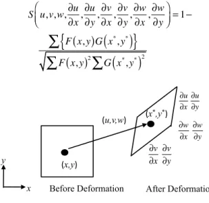
In the fine search of the DICM, deformation of each subset is estimated by iterative computation. Image of fine search is shown in Fig.2. The problem is to find the value of an appropriate subset deformation i.e., displacement and strain components, such that the highest correlation coefficient is obtained. To solve this problem, the performance function is defined as Eq. (2), which is necessary to obtain the appropriate subset deformation i.e., displacement and strain components u, v, w, !u !x^, !u !y^, !v !x^, !v!y, !w !x and !w !y, so as to minimize the performance function S.

S u,v,w,!u

!x,!u

!y,!v

!x,!v

!y,!w

!x,!w

!y

"

#$

%

&'=1(

F x,

( )

y ^{G x}

(

^*,y*

)

{ }

)

F x,

( )

y²

) )

^{G x}

(

^*,y*

)

²

(2)

!x,y"

!x^*,y^*"

!u,v,w"

!u

!x!!u

!y

!v

!x!!v

!y

!w

!x!!w

!y

x y

Before Deformation

After Deformation

Fig.2 Image diagram of fine search

where F(x, y) and G(x^*, y^*) are light value of specimen surface at before and after deformation. In addition, x^* and y^* are the point of (x^*, y^*) transferred from arbitrary point of (x, y), and those are expressed as Eq. (3).

x_i^*=x_i+u_i+!ui

!x"x+!ui

!y"y (3) where i=1, 2, 3, (x1, x2, x3)=(x,y,z) and (u1,u2,u3)=(u,v,w). In addition, ∆x and ∆y are distance between center point and target point in subset.

In this study, a steepest descent method is applied to solve this problem. The update equation with respect to unknown variables is shown in Eq. (4).

{ }

U ^{( )l+1} =

{ }

U ^{( )l} !"^{( )l #S}

$#U

%&

'( )

( )l

(4)

where

{ }

U ^{and "}#_!U^!S

$

%&

' are expressed as Eqs. (5) and (6).

{ }

U ^T = u,v,w,!u

!x,!u

!y,!v

!x,!v

!y,!w

!x,!w

!y

"

#$

%&

', (5)

!S

!U

"

#$

%&

'

T

= !S

!u,!S

!v,!S

!w, !S

! !u

!x

( )

^{,!,! !}

( )

^!Sw_!y

"

#(

$(

%

&

(

'( (6) where α is a step length, and l is the number of iteration.

Moving Least Square Method

In the MLSM, the interpolation function for unknown variable u(x) i.e. each component of displacement vector, is written as Eq. (7).

u x

( )

^=pT

( )

^{x a x}

( )

^{= pT}

( )

^{x A!1}

( )

^{x B x}

( )

^u=qT

( )

^{x u (7)}

where p^T

( )

x ^{and a x}

( )

are, basis function and unknown coefficient vector, a function of {1 x y} and {a0(x,y) a1(x,y) a2(x,y)}, respectively. q(x) is shape function, and A(x), B(x) and u are calculate by Eqs. (8) through (10).

A x

( )

= w r

( )

_i ^{p x}

( )

i ^pT

( )

^xi i=1

!

n (8)

B x

( )

=_"#w x

(

!x₁

)

^{p x}

( )

1 ^{,!w x}

(

^!xn

)

^{p x}

( )

n _$% (9) u^T =

{

u₁,u₂,!u_n

}

(10) where n is the number of evaluation nodes in domain of influence, and w(r_i), x and x_i are weighting function, coordinates at evaluation and reference nodes. In this study, two dimensional first order basis functions are applied to the shape function q(x) shown in Eq. (7). In addition, fourth order spline function shown in Eq. (11) is employed as a weight function.

w r

( )

_i ^=1.0!6.0 _r^ri

mi

"

#$

%

&'

2

+8.0 r_i r_mi

"

#$

%

&'

3

!3.0 r_i r_mi

"

#$

%

&'

4

(11)

where r_i and r_mi are the distance from x to x_i, and the radius of domain influence, respectively. Consequently, strain components εxx, ε_yy are calculated as Eq.(12).

!_xx="u

"x="

(

p^T

( )

x ^{a x}

( ) )

"x , !_yy="v

"y="

(

p^T

( )

x ^{a x}

( ) )

"y (12)

Element Free Galerkin Method

The equilibrium equation, the strain-displacement relation and the stress-strain relation are expressed as Eqs. (13), (14), and (15).

!_{ij. j}=0 (13)

!ij= 1

2

(

u_{i, j}+u_j,i

)

(14) !_ij=D_ijkl"_kl (15)

where σij, εij, u_i and D_ijkl are stress, strain, displacement and elastic modulus tensor, respectively. Where Eqs. (13), (14) and (15) are expressed in matrix forms as Eq. (16), (17) and (18).

[ ]

C ^T

{ }

^{! =}

{ }

⁰ , (16)

{ }

! ⁼

[ ]

^C

{ }

^u , (17)

{ }

! ⁼

[ ]

^D

{ }

^" (18) where [C], {σ }, {ε}, {u} and [D] are shown in Eq. (19), (20),

(21), (22) and (23), respectively.

[ ]

C ^{T =}

!!x 0 0 !

!y 0 !

!z

0 !

!y 0 !

!x !

!z 0

0 0 !

!z 0 !

!y !

!x

"

#

$$

$$

$$

%

&

'' '' ''

(19)

{ }

! ^T =

{

!_xx !_yy !_zz "_xy "_yz "_xz

}

(20)

{ }

! ^T =

{

!_xx !_yy !_zz "_xy "_yz "_xz

}

(21)

{ }

u ^{T =}

{

^{u v w}

}

(22)

[ ]

D ⁼

!+2µ ! ! 0 0 0

! !+2µ ! 0 0 0

! ! !+2µ 0 0 0

0 0 0 µ 0 0

0 0 0 0 µ 0

0 0 0 0 0 µ

"

#

$$

$$

$$

$$

%

&

'' '' '' ''

(23)

where λ and µ are Lame’s constants.

Multiplying weighting function {u^*} for both sides of equilibrium equation and integrating a domain Ωa yields Eq.

(24)

#

"_a

{ }

u^{* T}

^{[ ]}

^{C T}

^{{ }}

^{! d"=0}. (24) Applying the Green theorem to Eq. (24) yields

#

"a

{ }

u^{* T}

^{[ ]}

^{C T}

^{{ }}

^{! d"=}

#

$a

{ }

^{u* T}

^{{ }}

^{t d$} (25) where {t} is traction force vector, t_i=!ijn_j.

Substituting the stress-strain relation to Eq. (25) yields

"

!_a

{ }

u^{* T}

^{[ ]}

^{C T}

^{[ ]}

^D

^{[ ]}

^C

^{{ }}

^{u d!=}

"

#_a

{ }

^{u* T}

^{{ }}

^{t d#}. (26) If the weighting function {u^*} and displacement {u} at an arbitrary point x are interpolated by each values at referred

nodes in the domain Ω_a based on Galerkin procedure, the interpolation function for each values are written as Eq. (27).

{ }

u ^=q1

( )

x ^u1+q₂

( )

x ^u2+!+q_n

( )

x ^un=q^T

( )

x

{ }

^u (27) where q(x) is shape function, and n is the number of referred nodes in the domain. The shape function is determined by the MLSM, and linear basis and forth order spline functions are employed as the basis function and weighting function.

Applying the interpolation functions to the Eq.(26) yields _!

[ ]

k ^d!

{ }

^u

"

a ⁼

"

#a

^{{ }}

^{f d#} (28)

where a coefficient matrix at the left hand side and a vector at the right hand side are the stiffness matrix and external force, respectively. In addition, Γ_a is the boundary on domain Ω_a. The penalty function method is employed to the treatment of essential boundary condition.

Eigen analysis

The derivation of characteristic equation shown in the reference of Pegeau et. al. [6] is simply explained. In this formulation, the computational region is defined by spherical configuration whose radius r is r0, and the spherical coordinate system is introduced (See Fig.3). As the final form of the derived equation, the equation on the spherical surface is obtained. Therefore, the surface domain is divided into finite elements, and the computation for the characteristic equation is carried out. If displacements for each element are expressed by interpolation function shown in Eq. (47) and the interpolation function is substituted to equation of the principle of virtual work, a characteristic equation is finally derived as shown in Eq. (48).

y

x

z

r

^Q

r₀

!

O

"

#

#=-1

#=1

$

%

$=1

$=-1

%=1

%=-1

1 2 3

4 5 7 6

8

Fig.3 Spherical coordinate system for eigen analysis

u_i

(

r,!,"

)

⁼ _r^r

0

#

$%

&

'(

p

h_ku_ik

k=1

)

8 (29)

(

p²

[ ]

A ^+p

[ ]

^{B +}

[ ]

^C

) ^{{ }}

^{u =}

^{{ }}

⁰ (30) where u_i is expressed by u_ik. In addition, h_i indicates the shape function. In the Eq. (30), p indicates characteristic root and

vector {u} denotes superposed displacement vector in entire domain, and matrices [A], [B] and [C] represent the coefficient matrices derived by finite element procedure. The characteristic root p is obtained by solving the Eq. (30) based on eigen analysis. Relationship between the characteristic root and the order of singularity λ is expressed by λ=Re(p)-1. If the parameter λ is -1< λ<0, it is denoted that stress fields has a stress singularity. On the other hand, if the parameter λ ^{is 0<} λ^, it is denoted that the stress singularity disappears.

EXPERIMENTS

Experimental apparatus and specimens

Tensile test for a specimen, i.e., a silicon chip is bonded to the substrate with resin (Fig.4), is conducted using a small tensile test machine (Fig.5), and surface image of the specimen is taken by a laser microscope. In experiment, the geometry near the stress singular point affects the intensity of singularity, in particular the sharpness of vertex in Si chip, which is brittle and hard material, will influence on the zone size of stress singular field. Figure 6 shows a photograph of the vertex in Si

Si Chip 14mm Resin Substrate

34mm 12mm

Fig.4 Schematic view of specimen

Laser microscpe

Load cell Specimen Stepping motor

24mm

3kN

Fig.5 Small tensile test machine

Fig.6 Photograph of a vertex in Si chip

chip taken by scanning electron micrograph (SEM). Measuring curvature at the vertex from the photograph yields about 1µ^m.

Next, an effect of round vertex on the distribution of surface strain in a stress singular field is investigated using the 3D- EFGM.

Model for analysis in EFGM

Numerical analysis for specimen model (Fig.7) is carried out. Specimen model used in the numerical analysis is a half size one in experiment considering the symmetry of shape and boundary condition. In this analysis, strain singular field near the edge of interface in the specimen model is computed based on the EFGM. Cell model in the analysis is shown in Fig.8,

Si chip

Substrate Resin 7mm

17.5mm 0.6mm

3mm x

z y

Fig.7 Model for EFGM analysis

Fig.8 Distribution of cell for EFGM analysis

Si chip R

Resin z

x o

r φ

Fig.9 Cell distribution around the round corner

where the minimum length of cell is 1.5µm. The corner near the Si chip is enlarged as shown in Fig.9. Here, the curvature, R, at the vertex in the Si chip is varied from 0, 6.25. 12.5µm.

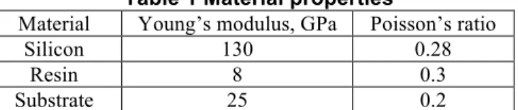
Strain distribution around the vertex near interface edge is computed in the enlarged region shown in Fig.9. Tensile stress of 10MPa is applied to the right end of the model shown in Fig.7. Material properties used in the analysis are shown in Table 1. Distribution of strain around the vertex on interface edge is shown in Fig.10. Figures 10(a) and 10(b) are distributions of εxx and εyy on the surface for R=0µm. As you can see these figures, large values of strains distribute along the interface between resin and Si. Figures 10(c) and 10(d) are the

Table 1 Material properties

Material Young’s modulus, GPa Poisson’s ratio

Silicon 130 0.28

Resin 8 0.3

Substrate 25 0.2

strain distributions for R=12.5µm. Comparing Figs.10(c) and

Si

Resin Substrate

7490 7495 7500 7505 7510 7515 7520 7525 7530 x , µm

320 325 330 335 340 345 350 355 360

z ,µm

0 0.0005 0.001 0.0015 0.002 0.0025 0.003 0.0035

φ o

z ,µm

x , µm (a) εxx (R=0µ^m)

7490 7495 7500 7505 7510 7515 7520 7525 7530 x , µm

320 325 330 335 340 345 350 355 360

z ,µm

-0.0005 -0.0004 -0.0003 -0.0002 -0.0001 0 0.0001 0.0002 0.0003 0.0004 0.0005

φ o

z ,µm

x , µm (b) εyy (R=0µ^m)

strain distribution for R=12.5mm. Comparing Figs.10(c) and (d) with Figs. 10(a) and 10(b), the distributions of εxx and εyy for vaguer than those for R=0mm. Now, we introduce a spherical coordinate system originated at a point on the interface between Si and resin as shown in Fig.9. All strain components are transformed from a rectangular system to the spherical coordinate system. Figure 11 represents the distribution of strain εφφ against the distance r from the origin on the interface.

Here, the angle φ for these plots is -45º. Red symbol indicates the result for R=0mm and shows the singular behavior against the distance r. In this analysis, the minimum size of cell is 1.5µm, so the plot less than 3µm looks like to be suppressed.

Green and Blue symbols represent the results for R=6.25µ^m and 12.5µm, respectively. As can be seen from this figure, the plots of εφφ for the round vertex bend around r=R. This means that when strain distribution in real joints depends on the curvature at the vertex and the intensity of singularity for strain might vary with the curvature.

5 6 7 8 9

10^-4

Strain

2 3 4 5 6 7 8 9

10 ^{2 3 4}

Distance r from point o , µm R m

0 6.25 12.5

(R=0)=2.33*10^-5r^-0.374+1.29*10^-4r^-0.307 1.03 (R=0)

1.1 (R=0)

Fig.11 Distribution strain εφφ against r Table 2 Order of stress singularity No. λ at vertex λ at singular line

Real part Real part Imaginary part

1 0.373711 0.228829 0

2 0.307088 0 0

Results of eigen analysis

3D eigen equation, Eq.(30), for the material combination of Si and resin is solved with respect to p and is determined the order of singularity, λ. Table 2 shows the values of the stress singularity. In this table, the orders of stress singularity for a vertex, and for a stress singular line are listed. For the vertex, there are 2 values yielding the stress singularity, which corresponds to power singularity. From eigen analysis, the strain singular fields can be expressed as:

!ij= A_kg_kij

( )

",# ^r$%k

k=1

&

2 (31)

where gkij(θ,φ) is the angular function of k^th order of singularity for strain εij. Coefficient A_k is the intensity of strain singularity.

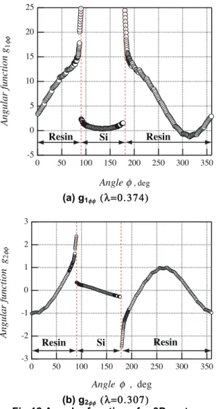
From the eigen analysis, eigen vector for each value of singularity can be obtained. In addition, angular functions for strain and stress fields can be calculated using eigen vector of displacement. Now, as examples, g_1φφ(π^/2,φ^{) and g}2φφ(π^/2,φ^{) for} vertex are shown in Fig.12. Furthermore, g_1φφ(π^/2,φ^{) for} singular line is shown in Fig.13. It is found that a typical mode for each order of singularity exists and strain fields under a general boundary condition are expressed by combining several power law terms including angular functions. As already shown, solid lines drawn in Fig.11 are represented lines obtained from Eq.(31).

7490 7495 7500 7505 7510 7515 7520 7525 7530 x , µm

320 325 330 335 340 345 350 355 360

z ,µm

0 0.0005 0.001 0.0015 0.002 0.0025 0.003

φ o

z ,µm

x , µm

(c) εxx (R=12.5µ^m)

7490 7495 7500 7505 7510 7515 7520 7525 7530 x , µm

320 325 330 335 340 345 350 355 360

z ,µm

-0.0005 -0.0004 -0.0003 -0.0002 -0.0001 0 0.0001 0.0002 0.0003

φ o

z ,µm

x , µm

(d) εyy (R=12.5µ^m)

Fig.10 Distribution of strain near the vertex in Si chip

25 20 15 10 5 0 -5 Angular function g1

350 300 250 200 150 100 50 0

Angle ^{, deg}

Resin Si Resin

(a) g_1φφ (λ=0.374)

-3 -2 -1 0 1 2 3

Angular function g2

350 300 250 200 150 100 50 0

Angle , deg

Resin Si Resin

(b) g_2φφ (λ=0.307)

Fig.12 Angular functions for 3D vertex

2.0 1.5 1.0 0.5 0.0

Angular function g1

360 300 240 180 120 60 0

Angle ^{, deg}

Resin Si

Fig.13 Angular function g_1φφ for singular line Strain field for R=0µm is expressed by a combination of two terms of power law. Strain near Si chip with the round vertex

decreases in a region r<R=6.25µm and 12.5µm, and strain distribution in R<r<1.5R is in parallel with the plot for R=0.

Furthermore, strain near the round vertex approaches the strain field for R=0µm near r=10-20µ^m.

Figure 14 shows the plots of strain εφφfor various angle φ near the Si vertex with R=0. Color plots represent the results of EFGM. In calculating strain near the interface, displacement data in Si, which is very small due to its rigidity, is used in our algorithm, hence strain values decrease near the vertex. So, we do not use the data near the vertex to determine the intensities of strain singularity, A_k, in Eq.(31).

5 6 7 8 9

10^-4

Strain

4 5 6 7 8 9

10 ^{2 3 4}

Distance r from point o , µm Angle , deg

250 260 270 280 290

2.33*10^-5+1.29*10^-4

Fig. 14 Strain plots for various angles of φ

200x10^-6

150

100

50

Intensity of singularity , Ak 0

300 290 280 270 260 250 240

Angle , deg

A₁ A₂

Fig.15 Determined intensity of singularity A₁ and A₂ Now, taking account of the distributions of angular function, g_kφφ, against φ, the coefficients A_k are determined for the plots in Fig.14 using a least square method. Straight lines drawn in Fig.14 are the approximated results for each plot.

Figure 15 represents the determined intensity of strain singularity. The values of Ak vary slightly with angle φ. Average values of each A_k are 1.44! 10^-5 and 1.19!10^-4, respectively.

Results in DICM

In experiment, strain distribution near the vertex is obtained using DICM analysis. In this section, method for determining the strain is described. In experiment, the tensile stress 2.17MPa (load:0.784N) is first applied to the specimen and 111.6MPa (load:40.18N) is further added. Figure 16 demonstrates photographs taken by a laser micrograph (OLYMPUS OLS4000 LEXT). A magnification is 1,080 times, and a size of one pixel is 0.130µm. Figures 16(a) and 16(b) are photographs before and after loadings, respectively. Si chip in these photographs locates at the right upper region. The size of DICM analysis is 19.5µ^m

!

^19.5µm, and the number of pixel is 150

!

150. The subset size used in DICM analysis is 30pixel

!

30pixel. Displacement field near the Si vertex is first determined by applying the image data of photographs to DICM. Figure 17 shows the relative displacement field near the Si vertex. In this figure, the origin of the displacement is located at the Si vertex. A large displacement can be observed in the resin. In the tensile test, the specimen deforms mainly in the x-direction. Figure 17 reflects the whole deformation in the

2 4 6 8 10 12 14 16 18

2 4 6 8 10 12 14 16 18

z ,µm

x , µm

Si

Resin

z , µm

x , µm

Fig.17 Displacement field near Si chip

(a) Before deformation

(b) After deformation Fig.16 Photographs near Si chip

"outputx0.5.dat"

2 4 6 8 10 12 14 16 18

x,µm 2

4 6 8 10 12 14 16 18

z,µm

-0.3 -0.2 -0.1 0 0.1 0.2 0.3

z , µm

x , µm Si

Resin

(a) εxx

"outputz0.5.dat"

2 4 6 8 10 12 14 16 18

x,µm 2

4 6 8 10 12 14 16 18

z,µm

-0.3 -0.2 -0.1 0 0.1 0.2 0.3 0.4 0.5

z , µm

x , µm Si

Resin

(b) εzz

Fig.18 Distributions of strain near Si chip

specimen.

Next, the moving least square method (MLSM) is applied to calculate strain fields using the displacement data obtained from the DICM analysis. In this analysis, the radius of domain influence is 1.5µm. The calculated strains εxx and εzz are shown in Fig.18. In particular, a large strain of εzz occurs along the lower interface of Si chip and resin. For εxx, a large value occurs along the vertical interface of Si chip and resin. Strain εφφcalculated from εxx, εzz and εxz obtained by the EFGM analysis and strain obtained from MLSM are shown in Fig.19.

It is found that the strain obtained from MLSM is fairly agreed with the strain for R=0 calculated by EFGM. Considering the angular functions and determining the coefficients A1 and A2

yields 8.29!^{10-5 and 1.35}!^10-3, respectively.

CONCLUSION

In this study, the displacement and strain fields by using the image analysis based on the DICM and the MLSM and the numerical analysis based on the EFGM were estimated.

Conclusions in this study are summarized as follows.

(1) Strain distribution calculated by EFGM near the vertex of the Si chip in the specimen was fairly well approximated by an equation obtained from eigen analysis. Radius at the vertex in the Si chip affected the strain distribution near the vertex.

(2) Appropriate distribution of strain could be computed using the displacement distribution obtained by the DICM using image data of a laser micrograph. The intensities of strain singularity, A1 and A2, for external stress of 111.6MPa were 8.29!^{10-5 and 1.35}!^10-3, respectively.

ACKNOWLEDGMENTS

This work was supported by "Program for High Reliable Materials Design and Manufacturing in Nagaoka University of Technology". We wish to thank you for Mr. Hiroyuki TANAKA at SUMITOMO BAKELITE CO., LTD for providing us specimen employed in this study.

REFERENCES

[1] H. Koguchi, K. Hoshi, 2012, “Evaluation of joining strength of silicon-resin interface at a vertex in 3D joint structures,” J. Electronic Packaging, June, Vol.134, Issue 2, 020902-1-020902-7.

[2] Pan, B., Asundi, A., Xie, H. and Gao, J., 2009, “Digital image correlation using iterative least squares and pointwise least squares for displacement field and strain field measurements,” Optics and Lasers in Engineering, Vol. 47, pp.865-874.

[3] Kirugulige, M.S., Tippur, H.V. and Denny, T.S., 2007,

“Measurement of transient deformations using digital image correlation method and high-speed photography: application to dynamic fracture,” Applied Optics, Vol. 46, pp. 5083-5096.

[4] Kurahashi, T. Yamada. K. and Koguchi, H., 2011,

“Measurement of Displacement and Strain Fields near Interface of Bonded Structure Based on Digital Image

Correlation Method Using Surface Configuration Data,”

International Conference on Advanced Technology in Experimental Mechanics, pp.1-10.

[5] Kurahashi, T., Ishikawa, A. and Koguchi, H., 2011,

“Evaluation of Intensity of Stress Singularity for 3D Dissimilar Material Joints Based on Mesh Free Method, 11th International Conference on the Mechanical Behavior of Materials,” Procedia Engineering, (2011), Vol.10, pp.3095- 3100.

[6] Belytschko, T. Lu. Y. Y. and Gu, L. 1994, “Element-free Garerkin methods,” Int. J. Num. Methods in Engineering, 37, pp.229-256.

[7] Bruck, H.A., McNeill, S.R., Sutton M.A. and Peters, W.H., 1989, “Digital image correlation using Newton-Raphson method of partial differential correction,” Experimental Mechanics, 29, pp.261-267.

[8] Pageau, S.S. and Biggers Jr, S.B., 1995, “Finite element evaluation of free - edge singular stress fields in anisotropic materials,” Int. J. Num. Methods in Engineering, 38, pp.2225- 2239.

[9] Md. Shahidal, I. and Koguchi, H., 2009, “Characteristics of Singular Stress Distribution at a Vertex in Transversely Isotropic Piezoelectric Dissimilar Material Joints,” Asian Pacific Conference for Materials and Mechanics, a132.

5 6 7 8 9

0.001

Strain

2 3 4 5 6 7 8 9

10 ^{2 3 4}

Distance r from point o , µ^m

R m

0 _R=0 6.25 1.1 R=0

12.5 1.03 _R=0 Result by MLSM '0.95 R=0

Fig.19 Plots of εφφobtained from DICM and EFGM