2003, Vol. 46, No. 3, 306-318
AN APPROXIMATION FOR A CONTINUOUS DATUM SEARCH GAME WITH ENERGY CONSTRAINT
Ryusuke Hohzaki Alan R. Washburn National Defense Academy Naval Postgraduate School
(Received May 24, 2001; Revised April 18, 2002)
Abstract This paper deals with a datum search game, where a target reveals his position (datum point) at a certain time (datum time) and a pursuer begins the search for the target by distributing his searching effort some time later. The target might move in the diffusive fashion from the datum point to evade his pursuer. His motion is restricted by its continuity in a two-dimensional space and constraints on its energy and maximum speed. The pursuer distributes searching effort to detect the evader under constraints on the amount of effort. A payoff is assumed to be the summation of searching effort weighted by the probability distribution of the target. In the previous paper, we formulated the problem as a single-stage two-person zero-sum game on continuous space and continuous time and proposed an upper bound and a lower bound for the value of the game. This paper extends the result and proposes an approximation for the value, noting that a constant-speed motion is crucial for the target.
Keywords: Search, game theory, datum search game, control, calculus of variations
1. Introduction
This paper deals with a datum search game, where a target reveals his position (datum point) at a certain time (datum time) and a pursuer begins the search for the target by distributing his searching effort some time τ later. The target might move in the diffusive fashion from the datum point to evade his pursuer. His motion is restricted by its continuity in a two-dimensional space and constraints on its energy and maximum speed. The pursuer distributes searching effort after time τ to detect the evader under constraints on the amount of effort. A payoff is assumed to be the integral of searching effort weighted by the probability distribution of the target over the entire search space. Because, in a so-called random search, the probability of detecting the target is estimated by an exponential function of the integral, the payoff function gives an index for the overall detection probability. In the previous paper[17], where energy constraint had been taken account of on the target motion for the first time, we formulated the problem as a single-stage two-person zero-sum game on continuous space and continuous time and proposed an upper bound and a lower bound for the value of the game. This paper extends the result and proposes an approximation for the value, noting that a constant-speed motion is crucial for the target.
In the rescue operation or military one in the ocean, there happen many search operations motivated by the datum information, which includes the datum point, the datum time and other data. The searcher makes efforts to detect the target and the target acts as the evader in the search. Koopman[13] put together the results of the military Operations Research by the U.S. Navy in the Second World War into a book. He already had studied the datum search where the target took a diffusive motion after randomly selecting his
course from the datum point. Meinardi[14] modeled the datum search as a search game. He considered the discrete model, in which the search was executed in discrete cell space at discrete time points. In order to solve the game, he investigated the target transition so as to make the probability distribution of the target as uniform as possible in the space any time. That is why his method is difficult to be generally applied to other datum search problems. The direct application of the datum search could be military operations such as the anti-submarine warfare. Danskin[2] dealt with the military operation game, where a submarine took fixed course and constant speed once at the beginning of the search while an anti-submarine helicopter chose points to dip a sonar. He found an equilibrium point, the target strategy of which was just the uniform distribution of speed on a so-called speed circle. Baston and Bostock[1] and Garnaev[4] discussed games to determine the best points of hiding a submarine and throwing down depth charges by an anti-submarine helicopter in a one-dimensional search space. Washburn’s work[16] was about a multi-stage game of target’s and searcher’s discrete motions, where the payoff was the total traveling distance until the coincidence of the target’s cell and the searcher’s cell and both players had no restriction on their motions. Kikuta[11, 12] studied a game with the payoff of traveling cost. Eagle and Washburn[3] worked on a single-stage game, where the payoff was defined as the summation of values determined by players’ positions each time. He assumed the constraints on the cells which both players were able to move to. In these studies, the searcher’s strategy was to choose his cells. But it could be to distribute searching effort in search space. For such a game named the search allocation game[5], a basic problem is to determine a point of hiding a stationary target and a distribution plan of searching effort. Nakai[15], and Iida, Hohzaki and Sato[9] researched such stationary target games with the payoff of the detection probability or the expected reward. For moving target games, there were Iida’s and Hohzaki’s works[6, 8, 10]. Hohzaki[7] proposed numerical methods to solve more generalized moving target games, where it is just required that the payoff is concave for the searcher strategy and linear for the target strategy.
In the previous studies about the datum search and the moving target search we just outline above, they did not set so many constraints on the capability of target motion. Even if they did, those were simple such as an upper limit on the target speed or the selection of target path among the preplanned ones. In our previous study[17], we took account of energy on the target motion, which made the problem more practical, e.g. problems with limited capacities of batteries and the energy consumption of players caused from waves on the sea or in the air. In continuous search space, there could be infinite number of feasible taget paths. Furthermore, the constraints on energy destroy the Markovian property of target motion, which makes the problem more complicated. Due to these reasons, we could not obtain optimal solution nor any optimal value for the game but proposed an upper bound and a lower bound of the game value. In this paper, we propose an approximation for the game value based on a constant-speed motion of the target, the importance of which will be clear later.
First of all, we describe assumptions of the problem and formulate it in the next section. In Section 3, we discuss the discrete modeling of the problem and emphasize that the constant-speed motion is crucial for the target strategy. We propose an upper bound and an approximation for the value of the continuous game based on the constant-speed motion in Section 4. Some numerical examples are illustrated in Section 5.
2. Description and Formulation of Datum Search Game
The datum search game was originally considered in a two-dimensional search space, which was regarded as the surface of the ocean or the land. In such a traditional way, we model a datum search game, which two players, a searcher and a target, take part in.
(1) The game is played in a two-dimensional continuous Euclidean space R2. Its origin is
the datum point which kicks off the datum search at time t = 0.
(2) After datum information is given, a searcher is dispatched to the datum area. He starts the datum search after time late τ and continues it until time T . The searcher can distribute the total amount ρ of divisible searching effort per unit time in the search space.
(3) The target is just at the origin at time t = 0 and moves on a plane R2. The usage of
speed v spends energy µ(v) per unit time. The function µ(v) is assumed to be convex and monotone increasing for v. The speed over maximum speed S is prohibited. The target possesses energy E at the initial time.
(4) Assuming that the probability of detecting the target at a point is proportional to the amount of searching effort distributed there, the integral of searching effort weighted by the target probability on the entire search space could be regarded as an index of the overall detection probability of the target. We adopt the integral as a payoff of the single-stage two-person zero-sum game. The searcher plays as a maximizer and the target as a minimizer.
Because the game is the point symmetric problem for the origin, we adopt distance x from the origin as the coordinate of Euclidean space. Using an indicator t for time, we denote the distribution density of searching effort at point x ∈ [0, ∞) and time t by h(x, t) and the probability density of the target resulting from the target motion by f (x, t). For the searcher’s strategy H = {h(x, t), x ∈ [0, ∞), t ∈ [τ, T ]} and the target’s strategy F =
{f (x, t), x ∈ [0, ∞), t ∈ [0, T ]}, the payoff is given as follows. G(H, F ) = Z T τ Z Xt h(x, t)f (x, t)2πxdxdt (1)
where Xt indicates the possible area of the target at time t. We have
R∞
0 h(x, t)2πxdx ≤ ρ, τ ≤ t ≤ T as the constraint of the searching effort. The probability density f (x, t) ≥ 0
depends on the target motion and has to satisfy RXtf (x, t)2πxdx = 1, 0 ≤ t ≤ T . On the
target motion, which is represented by position x(t) and velocity v(t) ≡ dx(t)/dt at time t, there are constraints v(t) ≤ S andR0T µ(v(t))dt ≤ E.
3. Discrete Modeling
Here we consider a discrete model of the original continuous game and find an optimal solution. Let T = {1, · · · , T } and K = {1, · · · , K} be time space and cell space, respectively, which are made by discretizing the original continuous space R2 and time space [0, T ].
The number of feasible target paths satisfying the energy constraint and maximum speed constraint is finite. We denote a set of feasible paths by Ω and target’s position of path
ω ∈ Ω at time point t by ω(t), and furthermore a set of paths passing through cell i ∈ K
at t by Ωt
i ≡ {ω ∈ Ω|ω(t) = i}. The searcher is able to consume searching effort up
to Φ(t) at time t after τ . The distribution of searching effort is represented by variables
{ϕ(i, t), i ∈ K, t = τ, · · · , T }, which is the searcher’s strategy. A mixed strategy of the
chooses a path ω out of Ω and totals one, Pω∈Ωπ(ω) = 1. By these notation, we can
formulate the payoff of the game as G(ϕ, π) =Pωπ(ω)PT
t=τϕ(ω(t), t), from which we have
max ϕ G(ϕ, π) = maxϕ T X t=τ X i X ω∈Ωt i π(ω) ϕ(i, t) =XT t=τ Φ(t) max i X ω∈Ωt i π(ω) .
Now to obtain the mini-max of G(ϕ, π) and an optimal strategy of the target, we only need to solve a linear programming problem PT.
(PT) min {ν(t),π(ω)} T X t=τ Φ(t)ν(t) s.t. X ω∈Ωt i π(ω) ≤ ν(t), i ∈ K, t = τ, · · · , T, π(ω) ≥ 0, ω ∈ Ω, X ω∈Ω π(ω) = 1 .
In another way, we can formulate the minimum of G(ϕ, π) with respect to π as follows. min π G(ϕ, π) = minω T X t=τ ϕ(ω(t), t) .
For the max-min of the payoff and an optimal strategy of the searcher, the following linear programming problem is to be solved.
(PS) max {µ,ϕ(i,t)} µ s.t. T X t=τ ϕ(ω(t), t) ≥ µ, ω ∈ Ω, X i∈K ϕ(i, t) ≤ Φ(t), t = τ, · · · , T, ϕ(i, t) ≥ 0, i ∈ K, t = τ, · · · , T.
Noting that problems PT and PS are dual each other, they give the same optimal value,
which is finite because the feasible regions of π and ϕ are bounded and the payoff can not be infinite. It gives the value of the game. Our discrete model is easy to be formulated. However we can imagine that the cardinality of feasible paths set Ω shows exponential increase for T and it causes the difficulties for solving the problem. In this paper, we have no intention to develop an efficient method to solve a large size of the discrete problem.
Next let us ask ourselves how far from the origin the target can reach each time. It is an important question since we can estimate the possible region of the target by its answer. Because, in the model of discrete time, the moving distance x between two consecutive time points indicates the velocity of the target at that time, the motion expends energy µ(x), which is a convex increasing function. There is also the maximum speed constraint x ≤ S. If we define fk(F ) as the longest distance by total energy F during k time points, we have
the following recursive formula.
fk+1(F ) = max
0≤e≤F {f1(e) + fk(F − e)}, f1(e) = µ
−1(e) . (2)
It results in fk(F ) = kµ−1(F/k) because we have
fk+1(F ) = maxe {f1(e) + fk(F − e)} = maxe
½ f1(e) + kf1 µ F − e k ¶¾ = max e (k + 1) ( 1 k + 1µ −1(e) + k k + 1µ −1 µF − e k ¶) ≤ max e (k + 1)µ −1 à e k + 1 + k k + 1 F − e k ! = (k + 1)µ−1 µ F k + 1 
by the mathematical induction and the concavity of inverse function µ−1(·). We can say that
the longest distance is accomplished by dividing the total energy equally into the number of opportunities of moving and successively carrying out the longest moving during two time points by the divided energy. Taking account of the maximum speed constraint, the longest distance fn(E) is given by
fn(E) = min{nµ−1(E/n), nS} . (3)
4. Estimation of the Value of Game for Continuous Model
At the end of the previous section, we discuss the expanding area of the target in the discrete time space, which is just the same as the continuous model. For the continuous game, the longest distance z(t) during time t is given by the following problem, where v(ξ) means target velocity at time ξ.
z(t) = max Z t
0 v(ξ)dξ s.t. 0 ≤ v(ξ) ≤ S, 0 ≤ ξ ≤ t, Z t
0 µ(v(ξ))dξ ≤ E . (4)
It is easily solved by the calculus of variations and an optimal solution is the constant speed
{v(ξ) = const, 0 ≤ ξ ≤ t}. What the target has to keep in mind is (1) expanding his possible
area as far as possible(Expanding strategy) and (2) distributing his probability as uniformly as possible(Uniformity strategy). The former strategy makes the density of searching effort thinner for the search to be less effective. The latter makes the searcher get confused about where he should focus his searching effort on. Usually, both are not compatible due to just the energy constraint. The target never always goes far to his reachable distance. The target who runs the longest distance in the early time stays there after then. The target who reaches to the farthest distance in the late time must be a slow starter since he can not run far in the early time.
From now, we outline the estimation of the lower bound and the upper bound for the value of the game, that we proposed in the previous paper[17], and then develop a new upper bound estimation and an approximation based on the constant-speed strategy.
By assuming that the target can accomplish both of the expanding strategy and the uniformity strategy, we estimate a lower bound for the value of the game. From (4), the longest distance at time t is given as follows.
z(t) = (
tS, 0 ≤ t ≤ E/µ(S)
tµ−1(E/t), E/µ(S) < t (5)
where µ−1(·) is an inverse function of µ(·). If the target can flatten his probability within
the radius z(t) for each time t, the resultant payoff GL gives us a lower bound for the value
of the game. GL= Z T τ ρ πz(t)2dt . (6)
Specifying a certain track of the target, we can estimate an upper bound of the game value. For any feasible track {y(t), 0 ≤ t ≤ T } of the target and its speed v(t) = ˙y(t), let the target take a speed profile W v(t) at time t, where W is a random variable on [0, 1] with probability density g(w) = 2w. His resultant probability distribution becomes uniform within a circle of radius y(t) each time t. The payoff becomes RτT ρ/(πy(t)2)dt. Therefore, let us find a
feasible track of minimizing the value. It is carried out by solving the following problem. min {v(t)} Z T 0 I(t)/y(t) 2dt s.t. v(t) = ˙y(t), 0 ≤ v(t) ≤ S, 0 ≤ t ≤ T,Z T 0 µ(v(t))dt ≤ E, (7)
where I(t) ≡ {0 if 0 ≤ t < τ ; 1 if τ ≤ t}. This problem is regarded as an optimal control problem for control vector v(t). Setting up the Hamiltonial function H(t) ≡ I(t)/y(t)2 + p(t)v(t) + λµ(v(t)) with multipliers p(t) and λ ≥ 0, we have some valid conditions to be
satisfied by optimal solution.
˙y(t) = ∂H/∂p = v(t), (8) ˙p(t) = −∂H/∂y = ( 0 if t < τ , 2/y(t)3 if τ ≤ t , and p(T ) = 0, (9) v(t) = arg min v(t) H(t) = S if p(t) ≤ −λµ0(S) , (µ0)−1(−p(t)/λ) if − λµ0(S) < p(t) < −λµ0(0) , 0 if − λµ0(0) ≤ p(t) , (10) Z T 0 µ(v(t))dt = E . (11)
p(t) is a negative and concave increasing function for t ≥ τ . From the monotone
increasing-ness of derivative µ0(·), we can say that optimal speed v(t) is monotone decreasing for time
t and is given by the following equation. Z v(t) V µ00(v) {H(b) + λ(vµ0(v) − µ(v))}3/2dv = − 2(t − b) λ (12)
where a pair of parameters (b, V ) is (τ, V ) of τ and V satisfying p(τ ) + λµ0(V ) = 0(Case
I) or (b, S) of b satisfying p(b) + λµ0(S) = 0 and S(Case II). Please refer to Appendix A to
verify the equation (12).
Now that we get an optimal track y∗(t) of the problem (7), an upper bound G1
U of the
value of the game is estimated by the following formula.
G1U =
Z T
τ
ρ
πy∗(t)2dt . (13)
Any feasible track gives us a boundary line, within which the target can arbitrarily form his probability distribution, not to mention the uniform distribution. The track {y∗(t), 0 ≤ t ≤
T } is the feasible track that gives the least payoff. But it neglects the strategy of combining
some feasible tracks. As seen before, the constant-speed motion gives the target the longest distance. The upper bound estimation that we are just going to propose is based on the combination of the feasible track y∗(t) and the constant-speed motion.
4.1. Upper bound estimation
It is known that the tracks randomized by the so-called triangular probability density of constant speed make the probability distribution of the target uniform on a plane. Here we consider a constant speed target diffusing in the randomized direction. The constant speed motion carries the target to the farthest distance each time as seen before. It gives us an idea that the target can secure some probability density near the boundary of his possible area by the mixed strategy of several constant speeds. Let g(v), vl ≤ v ≤ vu ≤ S be the
probability density of choosing constant speed v, where vl is a minimum speed and vu is
a maximum speed. Concerning with the probability density of the target at point x and time t, there are two kind of possible targets: one is just running there at speed x/t and another is staying after exhausting his energy. The latter possibility is obtained as follows. If the target just stops at time ν(≤ t), its speed must have been x/ν before stopping, which
equals x/η−1
E (x) from E = νµ(x/ν) or x = νµ−1(E/ν), where we define ηE(ν) ≡ νµ−1(E/ν).
Therefore, the probability density of target fE(x, t) at point x and time t is given by
fE(x, t) = 1 2πxtg(x/t) + ξE(x) 2πx g ³ x/ηE−1(x)´ (14) where ξE(x) ≡ −d ³
x/η−1E (x)´/dx. The first term f1(x, t) and the second term fE
2 (x) have different domains. f1(x, t) ≡ 1 2πxtg(x/t) , vlt ≤ x ≤ min{tµ −1(E/t), v ut}, (15) f2E(x) ≡ ξE(x) 2πx g ³ x/η−1E (x)´ , Evu µ(vu) ≤ x ≤ min{tµ−1(E/t), Evl/µ(vl)}. (16)
These terms are zero outside their respective domains. Letting h(x, t) be the distribution density of searching effort at point x and time t, we have
max {h(x,t)}G(H, F ) = {h(x,t)}max Z T τ Z tµ−1(E/t) 0 fE(x, t)h(x, t)2πxdxdt = Z T τ ρ0≤x≤tµmax−1(E/t)fE(x, t)dt (17)
from Equation (1). Now we are at the position to formulate the problem giving an upper bound G2
U of the value of the game.
G2
U = ming(v)
Z T
τ ρ 0≤x≤tµmax−1(E/t) fE(x, t)dt . (18)
In general, this optimization problem is difficult to solve. Instead, we can obtain other upper bounds by specifying the form of g(v) and optimizing parameters contained in it. As an example of g(v), we will take a linear function in Section 5
4.2. Approximation
An essential point that the target must keep in mind about his motion is to flatten his probability distribution as rapidly as possible and spread it as far as possible, which makes the searcher give up effective search by concentrating searching effort. We review the prop-erties of target strategies used for the estimation of the upper bounds. The constant speed motion affords the target the longest distance each time. The feasible track {y∗(t)} gives
him a flexible method to design his probability distribution in its interior area because it is just one of feasible paths and he can take a lot of tracks passing through in it. In result, this motion helps the target flatten his probability distribution. Therefore the composition of these motions is consistent with the essential point for the target as said above.
We assume that the target can move so that it combines the uniform probability density at point x of 0 ≤ x ≤ y(t), where y(t) represents the expanding radius derived from (7), with probability density fE(x, t) of (14) for y(t) ≤ x ≤ tµ−1(E/t) in the ratio of α(t) to
β(t). Now we have the total of the probability density, Z y(t) 0 α(t) πy(t)22πxdx + Z tµ−1(E/t) y(t) β(t)fE(x, t)2πxdx = 1 . (19)
Furthermore we require that the probability of the interior area is higher than one of the marginal area and then we have
α(t)
From Equations (19) and (20), the uniform density γ(t) in the interior area is given by
γ(t) ≡ α(t) πy(t)2 =
maxy(t)≤x≤tµ−1(E/t) fE(x, t) πy(t)2max
y(t)≤x≤tµ−1(E/t) fE(x, t) +
Rtµ−1(E/t)
y(t) fE(x, t)2πxdx
. (21)
Now the target shapes his probability density according to
f (x, t) = (
γ(t), 0 ≤ x ≤ y(t) ,
β(t)fE(x, t), y(t) ≤ x ≤ tµ−1(E/t) .
Letting Xt be the region in which the probability density is γ(t) at time t, we estimate an
approximation Gapx for the value of the game by maximizing the payoff function (1) with
the density f (x, t) with respect to {h(x, t)}.
Gapx = Z T τ Z Xt γ(t)h(x, t)2πxdxdt = Z T τ ργ(t)dt . (22) 5. Numerical Examples
In this section, we compare the estimations of GL, G1U, G2U and Gapx. First we derive more
concrete expressions for them from the theory in the previous sections by setting energy consuming rate µ(v) = v2. After that, we examine numerical examples by fixing parameters T, ρ and so on.
(1) Estimation of GL
Applying µ(v) = v2to Equations (5) and (6), we estimate the lower bound in three cases
depending on search period [τ, T ]. (i) In the case of E/S2 ≤ τ , G
L =
ρ
πElog(T /τ ).
(ii) In the case of τ < E/S2 < T , G
L = ρ πS2 Ã 1 τ − S2 E ! + ρ πE log T S2 E .
(iii) In the case of T ≤ E/S2, G
L = ρ πS2 µ1 τ − 1 T ¶ . (2) Estimation of G1 U
After defining a function l(x) by
l(x) ≡ 2E x s T − x T , log q T /(T − x) + 1 q T /(T − x) − 1 , (23)
we can derive optimal track y(t) and upper bound G1
U by (b, V ) of (I) b = τ and V =
q l(τ )
in the case of l(τ ) ≤ S2 or (II) b(> τ ) of l(b) = S2 and V = S in the case of l(τ ) > S2. Speed : v(t) = ( V, 0 ≤ t ≤ b V (T − t)qb/(T − b)/qT (T − b) − (T − t)2, b < t ≤ T (24) T rack : y(t) = ( V t, 0 ≤ t ≤ b Vqb/(T − b)qT (T − b) − (T − t)2, b < t ≤ T (25) Upper bound : G1U = ρ πV2 µ1 τ − 1 b ¶ + ρ πV2 1 2b s T − b T log q T (T − b) + (T − b) q T (T − b) − (T − b) . (26)
See the details in Appendix B. (3) Estimation of G2
U
The first step of estimating G2
U is to calculate some well-defined functions. These are
ηE(x) =
√
Ex, η−1
E (x) = x2/E, ξE(x) = E/x2 and so on. Let us adopt a linear density
function g(v) = av + b (0 ≤ v ≤ vu ≤ S, b ≥ 0) and find optimal parameters a, b, vu to
minimize the value (17). From Rvu
0 g(v)dv = 1, we have av2
u/2 + bvu = 1 . (27)
We can determine the function fE(x, t) using functions (15), (16) and t ≡ E/ve 2u, which is
the time when the target with speed vu exhaustes the initial energy E.
(i) In the case of t ≤ t, fe E(x, t) = (ax + bt)/(2πxt2) for 0 ≤ x ≤ v
ut. If b > 0, fE(x, t)
becomes infinity at x = 0. Therefore, b must be zero and then a is 2/v2
u. Consequently,
we have
fE(x, t) = 1/π(vut)2 . (28)
(ii) In the case of et ≤ t, fE(x, t) = ( 1/π(vut)2, 0 ≤ x ≤ E/vu , 1/π(vut)2+ E2/πv2ux4, E/vu ≤ x ≤ √ Et . (29)
Using fE(x, t), we compute maxhG(H, F ) of Equation (17) in the case of τ ≤ et ≤ T and
q E/T ≤ vu ≤ q E/τ to obtain max h G(H, F ) = Z et τ ρ πv2 ut2 dt + Z T et à ρ πv2 ut2 + ρvu2 πE2 ! dt = ρ π ( 1 v2 u µ1 τ − 1 T ¶ + T E2v 2 u ) − ρ πE .
Similarly, in the case of et ≤ τ and qE/τ ≤ vu,
max h G(H, F ) = ρ πv2 u µ1 τ − 1 T ¶ + ρvu2 πE2(T − τ )
and in the case of T ≤et and vu ≤qE/T ,
max h G(H, F ) = ρ πv2 u µ 1 τ − 1 T ¶ .
Now let us minimize maxhG(H, F ) with respect to vu in the above each case. Optimal
solutions of vu are v∗u =
q
E/τ and v∗ u =
q
E/T in the last two cases of qE/τ ≤ vu and
vu ≤
q
E/T , respectively. That indicates that the first case becomes a representative for
these two cases. For the first case, it is easily seen that optimal vu is α satisfying equation
(1/τ −1/T )/α2 = T α2/E2or α ≡ qE/T 4
q
T /τ − 1. Taking account of the domain of vu and
the maximum speed S, we obtain an upper bound G2
U classified into four cases. Optimal
density of target velocity is given by g(v) = 2v/v2
u, 0 ≤ v ≤ vu using vu posted for the
following each case.
(i) In the case of T /τ ≥ 2,
(a) if α ≤ S, vu = α and G2U = ρ πE 2 s T − τ τ − 1 ,
(b) if α > S, vu = S and G2U = ρ π ½ 1 S2 µ 1 τ − 1 T ¶ + T E2S 2 ¾ − ρ πE.
(ii) In the case of T /τ < 2, (a) if qE/T ≤ S, vu = q E/T and G2 U = ρ πE µT τ − 1 ¶ , (b) ifqE/T > S, vu = S and G2U = ρ πS2 µ1 τ − 1 T ¶ . (4) Approximation Gapx
It is enough for the estimation of Gapx to calculate γ(t) from the results of G1U and G2U.
By using y(t) of (25), fE(x, t) of (29) and optimal vu in the above discussion, in the case of
e
t ≤ t, we have
(i) if y(t) ≤ E/vu, maxy(t)≤x≤√EtfE(x, t) = 1/π(vut)2+ v2u/πE2 and
R√Et
y(t) fE(x, t)2πxdx =
1 − (y(t)/vut)2.
(ii) if y(t) > E/vu, maxy(t)≤x≤√EtfE(x, t) = 1/π(vut)2+E2/πv2uy(t)4and
R√Et
y(t) fE(x, t)2πxdx =
E2/v2
uy(t)2− y(t)2/v2ut2.
Rounding up the results of easy estimation in the case of t ≤t, we can itemize the expressione
for γ(t) as follows. γ(t) = min {1/(πv2 ut2), 1/(πy(t)2)} f or t ≤ E/v2u (E2+ v4
ut2)/{πvu2t2(E2+ y(t)2vu2)} f or t > E/vu2 and t ≤ t∗
(y(t)4+ E2t2)/(2πy(t)2t2E2) f or t > E/v2
u and t > t∗
where t∗ is the time that y(t∗) equals E/v
u and is given by t∗ = ( E/V vu if V b ≥ E/vu T −qT2− T b − (E/v u)2(T − b)/bV2 if V b < E/vu
with a pair (b, V ) of the estimation G1
U.
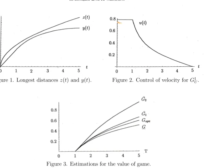
Now let us compare each estimation for fixed parameters ρ = 1, τ = 1, T = 5, E = 1, S = 5. We draw two tracks of the longest distance z(t) given by (5) and y(t) by (25), in Figure 1, where the abscissa indicates time and the ordinate the distance from the origin. After time t = 3, the gap between them is spreading time by time. Figure 2 shows the velocity of expanding motion Equation (24), in which we can see its decreasingness after being constant. Changing search time T from 1 to 5, we calculate GL, G1U, G2U and
Gapx and illustrate them in Figure 3 while other parameters are the same as the previous
example. Approximation Gapx lies between G1U and GL. But the error rate of G2U seems to
be comparatively large. The difference between G1
U and GL is affected directly by the gap
between y(t) and z(t).
6. Conclusions
In our previous paper, we revisited a datum search game on a two-dimensional plane, which Koopman started to consider in WWII first and we made the problem more practical by taking account of energy constraint on the target motion. For the continuous version of the problem, it seems to be difficult to find an optimal solution. We proposed some estimations for the value of the game: a lower bound, an upper bounds. In this paper, we added two estimation, an upper bound and an approximation by considering the constant-speed strategy of the target. The upper bound seems not to be a good estimation for the value of
Figure 1. Longest distances z(t) and y(t). Figure 2. Control of velocity for G1
U.
Figure 3. Estimations for the value of game.
the game, but the approximation lies between the upper bound and the lower bound. For the discrete version, we proposed a linear programming of giving optimal solution, although it have to be improved in order to cope with the so-called combinatorial explosion for large size of problems. In most of past similar researches, only the maximum speed of the target was limited. By comparing their results with ours, it will be clarified how much the energy constraint affects the game. In this paper, we take a simple payoff, which is bilinear for the evader’s probability distribution and the searcher’s distribution of searching effort. More complicated payoff, e.g. the probability of detecting the target adopted often in many search problems, will be able to be dealt with in the same manner. Some vehicles moving in the water or the air carry batteries to propel them. Some are accelerated by gasoline. If we give the rate µ(·) of energy consumption more practical forms for real engines, our model could be applied to more practical operations.
References
[1] V.J. Baston and F.A. Bostock: A one-dimensional helicopter-submarine game. Naval
Research Logistics, 36 (1989) 479–490.
[2] J.M. Danskin: A helicopter versus submarine search game. Operations Research, 16 (1968) 509-517.
[3] J.N. Eagle and A.R. Washburn: Cumulative search-evasion games. Naval Research
Logistics, 38 (1991), 495–510.
[4] A.Y. Garnaev: A remark on a helicopter-submarine game. Naval Research Logistics, 40 (1993) 745-753.
[5] A.Y. Garnaev: Search Games and Other Applications of Game Theory (Springer-Verlag, Tokyo, 2000).
[6] R. Hohzaki and K. Iida: A search game with reward criterion. Journal of the Operations
Research Society of Japan, 41 (1998) 629–642.
[7] R. Hohzaki and K. Iida: A solution for a two-person zero-sum game with a concave payoff function. In W. Takahashi and T. Tanaka(eds.): Nonlinear Analysis and Convex
Analysis (World Science Publishing Co., London, 1999), 157–166.
[8] R. Hohzaki and K. Iida: A search game when a search path is given. European Journal
of Operational Research, 124 (2000) 114–124.
[9] K. Iida, R. Hohzaki and K. Sato: Hide-and-search game with the risk criterion. Journal
of the Operations Research Society of Japan, 37 (1994) 287–296.
[10] K. Iida, R. Hohzaki and S. Furui: A search game for a mobile target with the con-ditionally deterministic motion defined by paths. Journal of the Operations Research
Society of Japan, 39 (1996) 501–511.
[11] K. Kikuta: A hide and seek game with traveling cost. Journal of the Operations
Re-search Society of Japan, 33 (1990) 168–187.
[12] K. Kikuta: A search game with traveling cost. Journal of the Operations Research
Society of Japan, 34 (1991) 365–382.
[13] B.O. Koopman: Search and Screening (Pergamon, 1980), 221-227.
[14] J.J. Meinardi: A sequentially compounded search game. In A. Mensh(ed.): Theory of
Games: Techniques and Applications (The English Universities Press, London, 1964),
285–299.
[15] T. Nakai: Search models wiht continuous effort under various criteria. Journal of the
Operations Research Society of Japan, 31 (1988) 335–351.
[16] A.R. Washburn: Search-evasion game in a fixed region. Operations Research, 28 (1980) 1290-1298.
[17] A.R. Washburn and R. Hohzaki: The diesel submarine flaming datum problem. Military
Operations Research, 6 (2001) 19-30.
Appendix A: Derivation of Equation (12)
We can verify Equation (12) as follows. The maximum principle tells us that conditions (8), (9) and v(t) = arg minv(t)H(t) hold. From ∂H/∂v = p(t) + λµ0(v(t)) and the monotone
increasingness of µ0(v), it is seen that ∂H/∂v changes in the range of [p(t) + λµ0(0), p(t) +
λµ0(S)] and then Equation (10) holds. If p(t) ≥ 0 for any t, it means v(t) = 0 any time.
Then it must be p(0) < −λµ0(0) ≤ 0. In case (I) of p(0) = p(τ ) > −λµ0(S), there must be
some V satisfying p(τ ) + λµ0(V ) = 0. It follows that v(t) = V for 0 ≤ t ≤ τ from (10). In
case (II) of p(0) = p(τ ) ≤ −λµ0(S), there is some b(> τ ) of p(b)+λµ0(S) = 0. It follows that
v(t) = S for 0 ≤ t ≤ b from (10). Noting that (µ0)−1(−p(t)/λ) decreases as time t increases,
we can see that v(t) decreases for t more than τ of case (I) or b of case (II). From now, the discussion proceeds only using b and V for simplicity. But we should not forget that b stands for τ in case (I) and V does for S in case (II). We can easily check that dH/dt = 0 and then H is constant for t ≥ b. Now we have H(t) = H(b) or
y(t)−2 = H(b) + λ(vµ0(v) − µ(v)) . (A–1)
If we can represent v = dy/dt by y from the above equation and consequently obtain
we differentiate both sides of (A–1) to obtain
µ00(v)
H(b) + λ(vµ0(v) − µ(v))3/2dv = −
2
λdt
or Equation (12). Equation (11) is self-evident. This equation and p(T ) = 0 help us decide parameters λ and H(b).
Appendix B: Estimation of G1
U in Section 5
Unless otherwise posted, a pair of parameters (b, V ) indicates (I) (τ, V ) of τ and V satisfying p(τ ) + λµ0(V ) = 0 or (II) (b, S) of b satisfying p(b) + λµ0(S) = 0 and S. At the
beginning, we can provide some functions µ−1(x) =√x, µ0(v) = 2v, (µ0)−1(x) = x/2. The
velocity v(t) stays being constant V and then y(t) = V t for 0 ≤ t ≤ b. For t ≥ b, we have
p(t) + 2λv(t) = 0. From Equation (A–1), we have
H(b) = 1/(bV )2− λV2 (B–1)
for t = b and a differential equation dy/dt = q1 − H(b)y2/(√λy), which is solvable as
follows. Z y(t) V b y q 1 − H(b)y2dy = Z t b dt √ λ .
The results are
y(t) = q λ − {λbV2− H(b)(t − b)}2 q λH(b) , (B–2) v(t) = s H(b) λ λbV2− H(b)(t − b) q λ − {λbV2− H(b)(t − b)}2 . (B–3)
Since v(T ) = −p(T )/(2λ) = 0, it must be λbV2 − H(b)(T − b) = 0. From this and (B–1), H(b) and λ are given by H(b) = 1/(T bV2) and λ = (T − b)/(T b2V4). Replacing H(b) and λ in (B–2) and (B–3), we obtain optimal speed (24) and track (25). Upper bound (26) is
given by calculation RτT ρ/(πy(t)2)dt.
After some calculations for equation (11), we obtain
bV2 2 s T T − blog q T /(T − b) + 1 q T /(T − b) − 1 = E .
This is helpful to check which of Case (I) or (II) is valid for the problem. Noting that function l(b) given by definition (23) is decreasing for b, we can see that Case (I) or (II) corresponds to l(τ ) ≤ S2 or l(τ ) > S2, respectively. All seems to be done.
Ryusuke Hohzaki
Department of Computer Science National Defense Academy 1-10-20 Hashirimizu, Yokosuka, 239-8686, Japan