A Multi - Objective Genetic Algorithm for Program Partitioning and Data Distribution Using TVRG

全文

(1)社団法人情報処理学会研究報告 IPSJ SIG Technical Report. 2004−MPS−50 (9) 2004／6／22. A Multi–Objective Genetic Algorithm for Program Partitioning and Data Distribution Using TVRG Masami Takata ∗ , Tomomi Yamaguchi † , Chiemi Watanabe † , Yoshimasa Nakamura ∗ ‡ , and Kazuki Joe † ∗. †. PRESTO, Japan Science and Technology Agency Kyoto University Kyoto-city, Japan. Graduate School of Humanity and Science Nara Women’s University Nara-city, Japan. Abstract We propose an algorithm that performs data distribution and parallelization simultaneously. The objectives of the algorithm are to reduce the length of critical path and the total memory size. Regardless to say, memory usage for each processor must be balanced. To obtain an optimal solution, we first adopted a branch and bound method. Since the branch and bound method often fails in the case of a large task graph, we adopt a multi–objective genetic algorithm, that provides a near optimal solution.. Keywords: Data distribution, Program partitioning, Parallel program, TVRG, Genetic algorithm, Multi– objective. 1. Introduction. To execute numerical simulations, we are working for the development of an automatic parallelizing compiler PROMIS-NWU [10]. It is an extension of PROMIS [8] developed at UIUC, which is also an automatic parallelizing compiler for shared memory environments. To design a parallelizing compiler for distributed memory environments, data distribution should be optimized as well as program partitioning of parallelization. Since both program partitioning and data distribution are known as an NP-complete problem [1], both problems should be solved simultaneously. TVRG (Task and Variable Representation Graph) [4] represents program flows and data dependence of given programs for PROMIS-NWU. To extract essential information from TVRG, given programs transform to an acyclic weighted direc-. ‡. Graduate School of Informatics Kyoto University Kyoto-city, Japan. tional task graph. In our previous works for program partitioning [5] [6], large task graphs can not be partitioned by branch and bound based approaches. Therefore, we assume that similar approaches for simultaneous partitioning to large task graphs also require too much computational resources. We here propose a GA (Genetic Algorithm) based simultaneous partitioning algorithm which provides a near optimal solution to given large task graphs. For an appropriate GA based algorithm, we use a multi–objective GA.. 2. Program Partitioning and Data Distribution. In TVRG [4], program flows are transformed into an acyclic weighted directional graph. Flow dependence and output dependence of data are also obtained as the node number information in the graph. Combining the acyclic weighted directional graph and data dependence, a task graph for our simultaneous partitioning algorithm is created.. 2.1. Definitions for Task Graphs. Program flows and data dependence are represented as an acyclic weighted directional task graph G = (N, E), where N and E indicate the sets of all nodes and edges of the task graph, respectively. Each n ∈ N corresponds to a task of a given program, and is assigned to a positive number (starting from 1). A function t(n) gives the cost required to execute the node n. An array Arn (l, m) expresses the range of an array elements accessed in the node n, where l shows the start (l = 0) and end (l = 1) element number and m indicates the array. An edge. −37−.

(2) 3. ni. Simultaneous Algorithm. Partitioning. The optimal partitioning is obtained by a BB–SP– algorithm (branch and bound based simultaneous partitioning algorithm), because the search space is expressed as a binary search tree. In the case Figure 1: Example of deadlock of large task graphs, the BB–SP–algorithm can not e = (ni , nj ) ∈ E (ni < nj ) indicates the existence give the optimal partitioning [5] [6]. An MOGA–SP–algorithm (multi-objective GA of data dependency from node ni to node nj , and based simultaneous partitioning algorithm) give the function c(e) gives the communication cost for near optimal solutions of the large task graph [9] the edge e, when node ni and nj are assigned to [7]. Since the genes correspond to the edges, the separate processors. results are sensitive to the coding mechanism of the 2.2 Definitions for Simultaneous genes. Therefore, we have proposed an edge sorting rule [7]. Partitioning In our simultaneous partitioning algorithm, the 3.1 BB–SP–algorithm number of possible edge conditions is 3: Inter-PE, We apply a BB–SP–algorithm to obtain three opIntra-PE, and U-E[2]. timal solutions which satisfy each objectives. The communication costs of Intra-PEs are conAt the initial setting of the BB–SP–algorithm, all sidered as zero. When a set of node Ni = edge states are U-E. Then, branch operations are {n1 , n2 , ...} connected Intra-PEP are merged, the to- performed repeatedly to generate the list of partial tal cost is given as t(Ni ) = ni ∈Ni t(ni ). The configurations. A partial configuration is expressed array access range is calculated as ArNi (0, m) = as a tuple < S, O >, where S contains the state minni ∈Ni Arni (0, m) (except Arni (0, m) = −1), information of all edges as an array, and O indicates and ArNi (1, m) = maxni ∈Ni Arni (1, m). In the the values of each objective as an array. case that a set of Inter-PE edges Ei = {ei 1, ei 2, ...} The procedure of the BB–SP–algorithm is sumare connected from the same node to Ni , the Ei marized as follows. 1. Generate a task graph G from TVRG. is said toPbe merged, and the cost is calculated as 2. Generate the initial configuration < S, O >, where each element of S is the U-E state. c(Ei ) = ei ∈Ei c(ei ). 3. Select a partial configuration < S 0 , O 0 > so that the minLet P = hn1 , n2 , ..., nm i be a path composed of imum critical path obtained from O 0 is included. 4. Examine whether each element of S 0 is not the U-E state. Inter-PEs and their sequentially connecting nodes • If no U-E edge remain, G0 is the first optimal par(i.e. there is an edge between ni and ni+1 where titioning. Go to step 8. 1 ≤ i < Pm). The cost • If there are U-E edges, choose an edge e0 whose P Tτ of P is given as state is U-E. Tτ (P ) = ei ∈alledgeswithinP c(ei ). ni ∈P t(ni ) + 5. Generate a partial configuration < S 01 , O 01 > by transforming the edge e0 state to Inter-PE. Create a graph G0 The critical path is defined as the path P so that with S 01 from G. Calculate O 01 of G0 . Add < S 01 , O 01 > Tτ (P ) is the largest. to the partial configuration list. The memory consumption of each node is cal6. Generate a partial configuration < S 02 , O 02 > by transP forming the edge e0 state to Intra-PE. Create a graph G0 culated as mem(n) = j (Arn (1, j) − Arn (0, j) + with S 02 from G. Examine whether G0 has deadlock. 1). Thus, the total memory consumption in a • If G0 does not have deadlock, Calculate O 02 of G0 . Add < S 02 , O 02 > to the partial configuration list. task graph G = (N, E) is given as M em(G) = P 7. Go to step 3. The maximum difference be8. Select a partial configuration < S 0 , O 0 > so that the minn∈N mem(n). imum M em(G0 ) from O 0 is included. tween memory consumption at each node of G 9. Examine whether each element of S 0 is not the U-E state. is defined as Ran(G) = (maxn∈N mem(n)) − • If no U-E edge remain, G0 is the second optimal (minn∈N mem(n)). partitioning. Go to step 12. • If there are U-E edges, choose an edge e0 whose The optimal solution must satisfy the following state is U-E. objectives: 1) Shorten the critical path length to re- 10. Execute the step 5 and 6. 11. Go to step 8. duce the parallel program execution time, 2) Min12. Select a partial configuration < S 0 , O 0 > so that the minimize the memory consumption M em(G), and 3) imum Ran(G0 ) from O 0 is included. 13. Examine whether each element of S 0 is not the U-E state. Minimize the maximum difference Ran(G). • If no U-E edge remain, G0 is the third optimal parFigure 1 shows the occurrence of deadlock. Obtitioning. The algorithm is terminated. viously, the graph is against the condition of an • If there are U-E edges, choose an edge e0 whose state is U-E. ’acyclic graph’. Therefore, solutions with deadlock 14. Execute the step 5 and 6. must be removed from search space. 15. Go to step 12. Inter-PE. nj. Intra-PE. −38−.

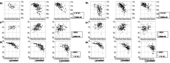
(3) 100(%). Table 1:. The optimal solution. (Using BB–SP–algorithm). object. max Tτ. M em(G). Ran(G). critical path length. 4683. 3873. 244. minimum M em(G). 14835. 1953. 440. minimum Ran(G). 7469. 3967. 207. 3.2. 80 60 40 20 0. MOGA–SP–algorithm. Chromosome:. 0. Each gene corresponds to an edge of a. 1. 2. Sorting0O. 3. 4. 5. 6. Ordering0A. 7. 8 9 10 (generation) Ordering1A. task graph. Hence, the length of the individual is ε(G). Since the edge condition is Inter-PE or Intra-PE, the individual {0, 1}. Crossover:. When multiple crossover points are employed,. the ratio of generating the deadlocked offspring may increase. Therefore, we adopt a single crossover point with the rate of 0.75. Two individuals are selected from the ancestor at random. The crossover point is selected at random.. Mutation:. The mutation rate is 0.01. For the mutation. operation, 5% of the individuals are selected and 20% of genes are flipped.. Fitness value:. Each individual has three kinds of fitness. values: the length of the critical path, M em(G) and Ran(G) of given task graphs expressed by the chromosome 01. Hence, an individual with smaller fitness values is better. If the given task graph has deadlock, we regard the fitness value of the individual as. P. n∈G. t(n) +. Process:. P. e∈G. c(e) + 1.. i) X = ε(G)2 individuals are generated.. ii). Select the superior X/6 individuals in each objective from ancestors, and copy them into a set Y , as the elitism strategy [3]. iii) Generate X ∗ 3/2 individuals by a crossover operation, and move them to Y . iv) Perform a mutation operation to Y . v) Calculate the fitness values in Y . vi) Select the superior X/3 individuals in each objective as the offspring. vii) Go to step ii.. 3.3. Sorting and Ordering. To make effective use of BB–SP–algorithm, the list of edges (e = (ni , nj )) is sorted by t(ni ) + t(nj ) + c(e) by descendent order [2]. On the other hand, we adopt Sorting 0O method proposed in [7] for MOGA–SP–algorithm. Since Sorting 0O depends heavily on the order of the nodes, we also use Ordering 0A or Ordering 1A [7]. Ordering 0A and Ordering 1A are an effective method for the reference of incoming and outgoing edges, respectively.. 4. Figure 2:. The ratio of the chromosomes with deadlock at each. generation. corresponds to {Intra-PE, Inter-PE }.. Experiments. We performed experiments for the evaluation of MOGA–SP algorithm. Experimental environment is: Linux 2.4.7 (RedHat Linux 7.1.2), Pentium 4 (1.8GHz) with memory capacity of 1GB. A task graph with 30 nodes and 29 edges are generated, because BB–SP– algorithm can not be executed in the case of larger. task graphs. Each node cost and edge cost are set to random numbers with a uniform distribution of [501, 1000]. The number of arrays used in the task graph is five, and each array has 100 elements. In MOGA–SP–algorithm, the generation count is 10. As the result, the execution times for BB–SP– algorithm and MOGA–SP-algorithm are 6.8[sec] and 0.9[sec], respectively. Table 1 shows the objective values for the optimal solution. To reduce M em(G), the accessed element size of arrays shared by different processors must be small. In a typical task graph, the range of the array elements used in a node overlaps to the other nodes. To decrease the overlapped area, those overlapping nodes should be merged in the same node. Consequently, the optimal solution for minimum M em(G) makes max Tτ increase. Hence, simultaneous partitioning algorithms must optimize the critical path length and the Ran(G) size, while the M em(G) size should be compromised by memory capacity. In MOGA–SP–algorithm experiments, we observe that individuals with deadlock exist at each generation. Figure 2 shows the ratio of individuals with deadlock. With all edge sorting methods, the number of individuals with deadlock decreases according to renewal operations. Consequently, the superior individuals with shorter critical paths increase by renewal. Figure 3, 4, and 5 show distributions of individuals without deadlock at each generation. In (b), the fitness values of each individual at the 10th generation are closer to the initial than at the initial generation. In (c), M em(G) increases and Ran(G) decreases at the 10th generation. Compared with the experimental result of BB–SP–algorithm, the optimal solution for critical path is also an approximate solution for Ran(G), and the optimal solution for Ran(G) has smaller critical paths than for M em(G). Therefore, at the 10th generation, several individuals are similar to the optimal solutions by BB–SP–algorithm. Con-. −39−.

(4) (a). 4700 8900 13100 17300 21500. (b). (c). 4300. 4300. 4300. 4300. 4300. 4300. 3600. 3600. 3600. 3600. 3600. 3600. 2900. 2900. 2900. 2900. 2900. 2900. 2200. 2200. 2200. 2200. 2200. 2200. 1500. 1500. 1500 CriticalPath. 1500. 1500. 1500 CriticalPath. 4700 8900 13100 17300 21500. 4700 8900 13100 17300 21500. 470. 470. 470. 380. 380. 380. 290. 290. 290. 200. 200. 200. 4700 8900 13100 17300 21500. 4700 8900 13100 17300 21500. (a). Mem(G). Ran(G) CriticalPath 4700 8900 13100 17300 21500. 200. 4700 8900 13100 17300 21500. Ran(G) CriticalPath 4700 8900 13100 17300 21500. 290. 290. 200 1500 2200 2900 3600 4300. 200 1500 2200 2900 3600 4300. 0 generation. 5 generation. 200 1500 2200 2900 3600 4300. 200 1500 2200 2900 3600 4300. 0 generation. 5 generation. Ran(G) Mem(G). 10 generation. The fitness values for each chromosome without deadlock. (Using Sorting 0O.) 4300. 4300. 4300. 3600. 3600. 3600. 2900. 2900. 2900. 2200. 2200. 2200. 1500. 1500. 1500. 4700 8900 13100 17300 21500. 470. 470. 470. 380. 380. 380. 290. 290. 290 200. Mem(G) CriticalPath. Ran(G) CriticalPath 4700 8900 13100 17300 21500. 470. 470. 470. 380. 380. 380. 290. 290. 290. 200 1500 2200 2900 3600 4300. 200 1500 2200 2900 3600 4300. 200 1500 2200 2900 3600 4300. 0 generation. 5 generation. Ran(G) Mem(G). 10 generation. Figure 4:. The fitness values for each chromosome without deadlock. (Using Ordering 0A.). sequently, we find our MOGA–SP algorithm is effective. In Figure 3 (a), we observe that the initial individuals have similar characteristics only when applying the Sorting 0O method. In general, the initial individuals in GA should start from difference conditions [3]. At the 10th generation by Ordering 0A and Ordering 1A, a lot of approximate solutions, in which the critical path length and the Ran(G) size decrease and M em(G) size increases, are observed. Thus, Ordering 0A and Ordering 1A methods are both effective for MOGA– SP–algorithm.. 5. 290. 200. 380. (c). Figure 3:. (c). 290. 200 4700 8900 13100 17300 21500. 290. 200 1500 2200 2900 3600 4300. 4700 8900 13100 17300 21500. 290. 380. 200 1500 2200 2900 3600 4300. 200. 380. 290. 290. 4700 8900 13100 17300 21500. 380. 380. 380. 290. 200. 380. 380. 380. 4700 8900 13100 17300 21500. 470. 470. 470. 4700 8900 13100 17300 21500. 4700 8900 13100 17300 21500. 470. 470. 470. (b). 4700 8900 13100 17300 21500. 470. 470. 470. (a). 4700 8900 13100 17300 21500. (b). Conclusions. In this paper, we proposed BB–SP–algorithm and MOGA–SP–algorithm for simultaneous partition-. Mem(G). Ran(G) Mem(G). 10 generation. Figure 5:. The fitness values for each chromosome without deadlock. (Using Ordering 1A.). ing of program partitioning and data distribution. Using the BB–SP–algorithm, we obtained the optimal solution in the case of 29 edges or below. Using the MOGA–SP–algorithm, a larger task graph can be partitioned approximately. We also validated Ordering 0A and Ordering 1A as effective ordering methods for the MOGA–SP–algorithm.. References. [1] M. R. Garey, D.S. Johnson. Computers and Intractability, A Guide to the Theory of NP-Completeness. W. H. Freeman and Company, San Francisco, California, 1979. [2] M. Girkar, C. D. Polychronopoulos. Partitioning Programs for Parallel Execution. Proc. of the 1988 Int. Conf. on Supercomputing, pp.216–229, 1988. [3] D. E. Goldberg. Genetic Algorithms in Search, Optimization, and Machine Learning. Addison-Wesley, 1989. [4] M. Haneda, H. Shouno, K. Joe. An Intermediate Representation for Parallelizing Compilers for DSM Systems. The International Workshop on Advanced Compiler Technology for High Performance and Embedded Systems, pp.47– 55, July, 2001. [5] M. Takata, Y. Kunieda, K. Joe. Accelerated Program Partitioning Algorithm - An Improvement of Girkar’s Algorithm. Proc. of the Int. Conf. on Parallel and Distributed Processing Techniques and Applications, Vol.II, pp.699–705, June, 2000. [6] M. Takata, Y. Kunieda, K. Joe. A Heuristic Approach to Improve a Branch and Bound based Program Partitioning Algorithm. The proceedings of the 1999 International Workshop on Innovative Architecture, pp.105–114, November, 2000. [7] M. Takata, H. Shouno, K. Joe: An Improvement of Program Partitioning Based Genetic Algorithm. The proceedings of the International Conference on Parallel and Distributed Processing Techniques and Applications (PDPTA ’02), Vol.I, pp.215–221, June, 2002. [8] H. Saito, N. Stavrakos, C. D. Polychronopoulos, A. Nicolau. The Design of the PROMIS Compiler. Int’l J. of Parallel Programming, Vol.28, No.2, pp.195–212, 2000. [9] T. Saito, T. Nakanishi, Y. Kunieda, A. Fukuda. Genetic Algorithm Based Program Partitioning. Proc. of the Int. Conf. on Parallel and Distributed Processing Techniques and Applications, Vol.II, pp.707–712, June, 2000. [10] T. Yamaguchi, H. Ishiuchi, A. Iwasaka, M. Haneda, H. Shouno, K. Joe. The Overview of the Paralleilzing Compiler PROMIS-NWU. Proc. of IPSJ SIGARC 2001-14414, pp.79–84, July, 2001. (in Japanese). −40−.

(5)