Subgrid-scale
energy
transfer
と渦層
渦管
東工大工学部
堀内
潔
1
Introduction
Large-eddy simulation (LES) is a turbulence simulation method in which the large scale (grid scale) field is directly calculated, while the small scale (subgrid-scale or SGS) field is modeled. The velocity and pressure fields $(f)$ are decomposed into grid-scale component
$(\overline{f})$ and SGS component $(f’=f-\overline{f})$ using a filtering procedure:
$\overline{f}(\mathrm{x})=\int_{-\infty}^{\infty}f(\mathrm{x})’\overline{G}(\mathrm{X}, \mathrm{x}^{l})d\mathrm{x}’$, (1)
where $\overline{G}(\mathrm{x})$ denotes the filter $\mathrm{f}_{\mathrm{U}11\mathrm{c}\mathrm{t}}\mathrm{i}\mathrm{o}\mathrm{n}$.
The effects of the SGS field on the grid-scale field is represented by the SGS stress
tensor, $\tau_{ij}=\overline{u_{?}u_{j}}-\overline{u}_{i}\overline{u}j$, which results from filtering the Navier-Stokes equations, where
$u_{i}’=u_{i}-\overline{u}_{i}$. The energy transfer between the grid scale field and the SGS field occurs
through the SGS production $\mathrm{t}\mathrm{e}\mathrm{r}\mathrm{l}\mathrm{n},$ $P=-\tau_{ij}\partial\overline{u}_{i}/\partial x_{j}$. When $P$ is Ilon-negative, the grid scale energy is forwardly transferred into SGS ($\mathrm{f}\mathrm{o}\mathrm{l}\cdot \mathrm{w}\mathrm{a}\mathrm{r}\mathrm{d}$ scatter), while if $P$ is negative the SGS energy is in turn transferred backwardly into the grid scale (backward scatter). Recent direct assessment of the energy transfer carried out using DNS data for wall-bounded flows $\perp,$ $2,3,4$)
revealed thatthe energy exchange is not unidirectional. Although
alnean direction ofenergy transfer is from the grid scale to the SGS, SGS energy is also
transferred in the opposite direction to the grid scale.
One of advantages of LES is that it can estimate an energy cascade from the given scale down to the slnaller scales locally in the physical space via the SGS production
term, enabling a detection of events which provides intense energy transfer. Coherent
structures are known to exist in the wall-bounded and free shear turbulent flows such as
the streaks in the former and the rib vortices in the latter. The objective of the present study is to investigate a correlation oi these coherent structures with the SGS energy transfer mechanism by utilizing the direct numerical simulation (DNS) flow fields (Sec. 2). A particular emphasis is placed on the backward scatter effect. In Sec. 3, the time development of the educed coherent structure is pursued $\mathrm{i}\mathrm{I}1$ the actual LES.
2
Eduction
of
intense
SGS
energy
production
events
In this section, we educe the structures associated with the generation of intense SGS energy using a conditional averaging $1\mathrm{l}\mathrm{l}\mathrm{e}\mathrm{t}\mathrm{h}_{\mathrm{o}\mathrm{d}}$.
2.1
Channel fiow
The wall-bounded turbulence DNS data that we used were for fully developed
incompress-ible channel flow with $Re_{\tau}$ (Reynolds number based on the wall-friction velocity,
$u_{\tau}$, and
the half channel height, $\delta$) $=180$. The Fourier-Chebyshev polynomial
expansion method
was used with 128, 129 and 128 grid points, respectively, in the $x,$ $y$ and $z$ directions. 5, 6)
In the following, $y_{+^{\mathrm{d}\mathrm{e}\mathrm{n}\mathrm{o}\mathrm{t}\mathrm{e}}}\mathrm{s}$ the wall coordinate$u_{\mathcal{T}}y/\nu$, where $\nu$ is the$\mathrm{k}\mathrm{i}\mathrm{n}\mathrm{e}\mathrm{n}_{\grave{1}}\mathrm{a}\mathrm{t}\mathrm{i}\mathrm{c}$viscosity. The channel flow field was filtered to 32 $\cross 129\cross 32$ in the $x,$ $y$ and $z$ directions,
respectively. In the filtering procedure described in Eq. (1), the $1\overline{1}\overline{1}o\mathrm{s}\mathrm{t}$ conumon filters are Gaussian, top-hat and spectral cutoff filters. In the present study, we adopted the Gaussian filter because this filter has a localizedsupport in physical space, which property is beneficial for the use of the scale-similarity model that we incorporate into actual LES. In the present work, no filter was applied in the $\mathrm{i}\mathrm{n}\mathrm{h}_{01\mathrm{n}\mathrm{o}}\mathrm{g}\mathrm{e}\mathrm{n}\mathrm{e}\mathrm{o}\mathrm{u}\mathrm{S}$ direction, but the same numerical discretization method was used in the inhomogeneous direction both in the direct $\mathrm{n}$-umerical simulation (DNS) data generation and in the LES
$\mathrm{c}\mathrm{o}1_{-}11\mathrm{p}\mathrm{u}\mathrm{t}\mathrm{a}\mathrm{t}\mathrm{i}\mathrm{o}\mathrm{n}\mathrm{S}$ . Numbers of LES grid points were chosen so that the turbulent kinetic energy retained in
the SGS components was large.
Figures 1 shows the $\mathrm{t}/$-distributions for plane-average of the individual terms in $P,$
$P_{ij}$
(no $\mathrm{s}\mathrm{u}\mathrm{m}\mathrm{n}\mathrm{l}\mathrm{a}\mathrm{t}\mathrm{i}_{0}\mathrm{n}$in $i$ and $j$), in which
$\tau_{xj}$ is estimated from
$\cdot$the exact SGS stress $\mathrm{o}\mathrm{b}\mathrm{t}\mathrm{d}\mathrm{i}_{\mathrm{I}}1\mathrm{e}\mathrm{d}$ from the channel flow DNS data. These terms were decolllposed into two-parts which
contribute to forward and backward scatters. Significant backward scatter arises in the normal production term of $P_{1\perp}$ term at $y_{+}\approx 15$. It can be seen that the
$\mathrm{n}\overline{\perp}$agnitude of forward and backward scatter termsin $P_{\perp\perp}$ is very close each other, wvith the total
sunl of
$P_{11}$ being slightly positive, but the sum even becoll\‘ies negative in the region
at $y_{+}\approx 12$.
Subsequently, the $\mathrm{r}\mathrm{o}\mathrm{o}\mathrm{t}_{- \mathrm{m}\mathrm{e}}\mathrm{a}\mathrm{n}-\mathrm{s}\mathrm{q}\mathrm{u}\mathrm{a}\mathrm{r}\mathrm{e}(\mathrm{r}\mathrm{m}\mathrm{s})$ value of$P_{11}$ termshowed a largest value among
the $P_{ij}$ terms, and the rmsvalues wereseveral times larger than the average values (figure
not shown).
The shear production term, $P_{12}$, is $\mathrm{d}\mathrm{o}\mathrm{n}$
)$\mathrm{i}\mathrm{n}\mathrm{a}\mathrm{n}\mathrm{t}$
in the very vicinity of the wall $(y_{+}<10)$.
The energy transfer arising in this ternl is predominantly forward due to the presence of
the large meanvelocity gradient near the wall. 1,4, 6) When the mean velocity gradient was
subtracted from the estimate of$P_{12}$ term, its $\mathrm{n}\overline{1}$agnitude was substantially reduced. Thus, the local variation of energy exchange between $\mathrm{g}_{\mathrm{T}}\mathrm{i}\mathrm{d}$ scale and SGS is better represented by $P_{11}$ term rather than $P_{12}$ or $P$ terms. It can be considered that $P_{11}$ ternl is nlore
appropriate to use for the detection ofthe events associated with intense grid scale-SGS energy transfer.
Based on above observations, we educe the coherent structures by sampling the events with intense $P_{11}$ term by applying a conditional averaging procedure. $\mathrm{L}1.7$)
The velocity fields were averaged for the events that corresponded to strong forward and backward
scatters in $P_{11}$ term. Strong forward scatter event was detected by
$\mathrm{i}_{111}\mathrm{p}\mathrm{o}\mathrm{s}\mathrm{i}\mathrm{n}\mathrm{g}$ the one-point conditions of the type $T(p_{t})>0.1_{\mathit{1}}$. where $T( \int J’)$ is defined as
$T(p_{t})= \int_{pt}^{\infty}fP(f)df//-\cdot\infty\infty|.fP(f)|(lf$. (2)
Here, $P(f)$ denotes the probability $\mathrm{f}\mathrm{u}\mathrm{n}\mathrm{c}\cdot \mathrm{t}\mathrm{i}\mathrm{o}\mathrm{I}\mathrm{l}$ of
$P_{\perp\perp}$. $\mathrm{S}\mathrm{i}_{111}\mathrm{i}\mathrm{l}\mathrm{a}\mathrm{r}\mathrm{l}\mathrm{y}$, for the $\mathrm{b}\dot{\mathrm{c}}\mathrm{L}\mathrm{c}\mathrm{k}\mathrm{w}\mathrm{a}\mathrm{r}\mathrm{d}$
event, the conditions of$T(p_{t})<-0.1$ was imposed, where $T(p_{t})$ is
$T(p_{t})= \int_{-\infty}^{p\iota}.fP(f)df/\int_{-\infty}^{\infty}.|fP(f)|df$. (3)
This detection was carried out for the grid points in the $x-z$ plane located at $y_{+}=12$.
It was felt that when an excessive symmetry is $\mathrm{i}\mathrm{n}$
)$\mathrm{p}\mathrm{o}\mathrm{s}\mathrm{e}\mathrm{d}$ for the conditional averaging, important fine structures are eliminated by superposing the structures with opposite ori-entations.
In theprevious analysis of the vorticalstructuresin thechannel, 8) itwas reported that
the histograms of $\theta$, inclination angle to the $x-z$ plane of the projection of the vorticity
vector in the $x-y$ planes, $\theta=\tan^{-1}(\overline{\omega}_{\underline{9}}/\overline{\omega}_{1})$ , was concentrated
$\mathrm{a}\mathrm{r}\mathrm{o}\mathrm{u}\mathrm{n}\mathrm{d}\pm 90^{\mathrm{o}}$ in the $x-z$
plane locatedat $y_{+}=12$. Here, $\overline{\omega}_{2}$ denotes the GS normal vorticity$\overline{\omega}_{2}(=\partial\overline{u}/\partial Z-\partial\overline{w}/\partial \mathcal{I})$ . This result indicates a significant contribution of the wall-normal vorticity for the vortex dynamics in the near wall region. In fact, the intensity of the shear production term of
$P_{13}$ shown in Fig. 1 is not negligible.
In order to eliminate the imposition of excessive$\mathrm{s}\}^{r}\mathrm{n}_{\overline{1}}\mathrm{m}\mathrm{e}\mathrm{t}\mathrm{r}\mathrm{y}$, we further constrained the
orientation of wall normal vorticity, i.e., the events with positive wall-normal vorticity
$\overline{\omega}_{arrow}9>0$ was chosen. Each time an event was detected, the whole grid scale velocity field
was stored, centering on the event. All the realizations where the condition was satisfied were then averaged to yield the conditionally-averaged fields. 7) Detection was done for both lower and upper walls. Approximately 150 events with large positive $P_{1\perp}$ term value
and a positive normal vorticity were detected and averaged from the 10 realizations of
the DNS data separated by non-dimensional tillle interval $0.6tu_{\tau}/\delta$.
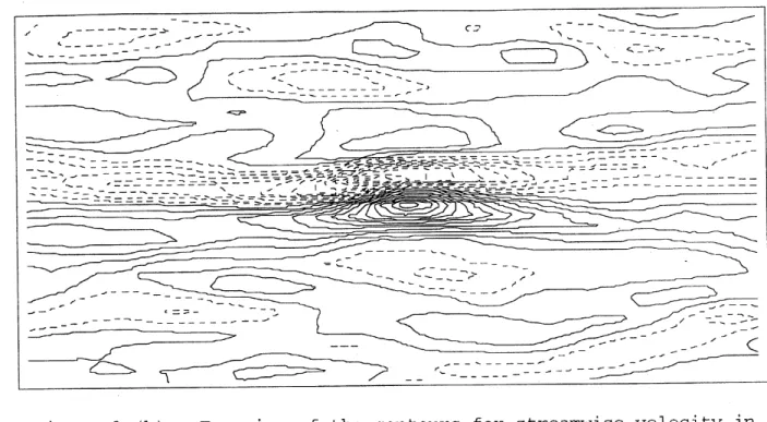
Figure 2 shows the contours of the streamwise velocity, $\overline{u}’’=\overline{u}-<\overline{u}>$
;
in the $x-z$plane at $y_{+}\approx 12$, associated with the detected events. $<f>$ denotes the average of $f$
in the $x-z$ plane. Positive values are plotted by the solid lines, and the negative ones
by the dashed lines. The flow is from left to right of the figure. Figures 2 (a) and (b)
show the results obtained from the forward-scatterevents $(T(p_{t})>0.1)$ (referred to asthe
$P_{11}$-Forward event) and the the backward-scatterevents $(T(p_{t})<-0.1)(P_{\perp\perp}$-Backward
event), respectively. These contours show asynunetric streaky structures. In Fig. 2 (a),
the region with negative contours (low speed streak) is $\mathrm{p}_{\mathrm{J}}1.\mathrm{a}\mathrm{c}\mathrm{e}\mathrm{d}\mathrm{d}_{\mathrm{o}\mathrm{W}\mathrm{n}\mathrm{S}}\mathrm{t}\mathrm{r}\mathrm{e}\mathrm{a}\mathrm{n}1$ of that with positive contours (high speed streak) near the detection polnt located at thecenter of this
$x-z$ plane. This result is similar tothose obtained in Johansson et al. 10) using the VISA
method and also those obtained using the $\lambda_{2}$ method in Jeong et al. 11).
To examine the accuracy of the educed flow field for an $\mathrm{a}\mathrm{p}\mathrm{p}\mathrm{r}\mathrm{o}\mathrm{X}\mathrm{i}\mathrm{n}\mathrm{l}\mathrm{a}\mathrm{t}\mathrm{i}_{\mathrm{o}\mathrm{n}}$ of the “real”
turbulence, the $y$-profiles of the grid-scale turbulence intensities are shown in Fig. 3,
in which the intensities are compared with those obtained fronl the ‘
exact’ filtered-DNS data. Although these intensities decay llluch faster as the distance fronl the lower wall is increased, because the vortical structures in the upper half of the channel were
smeared out, the overall intensity profiles are well represented $\mathrm{q}\mathrm{u}\mathrm{a}\mathrm{l}\mathrm{i}\mathrm{t}_{C}1\mathrm{t}\mathrm{i}\backslash ’\cdot \mathrm{e}\mathrm{l}\mathrm{y}$ . It should be noted that, quantitatively, the alnplitude of the intensities for the educed flow field is approximately a quarter of the filtered DNS data. This is because the significant $\mathrm{p}\mathrm{o}\mathrm{r}\iota \mathrm{i}\mathrm{o}\mathrm{l}\mathrm{l}$ of educed structure is concentrated near the detection poillt.
In the $P_{11}$-Forward event, a strong shear is generated $\mathrm{i}\mathrm{I}1$ the region where a high speed streak catches up with alow speed streak. This region coincides with the detection
point, where a large negative value for the longitudinal velocity derivative $\partial\overline{u}/\partial x$ occurs.
A large wall normal vorticity, $\overline{\omega}_{2}$, is generated in this region.
In the$P_{11}$-Backward event,alow speed streak is placed upstream of high speed streak
as shown inFig. 2 (b). Alarge positive value for the longitudinal velocityderivative$\partial\overline{u}/\partial x$
occurs in the region where a lowspeed streak resides adjucent to a high speed streak, and a large streamwise vorticity, $\overline{\omega}_{1}(=\partial\overline{w}/\partial y-\partial\overline{v}/\partial z)$ , is generated here.
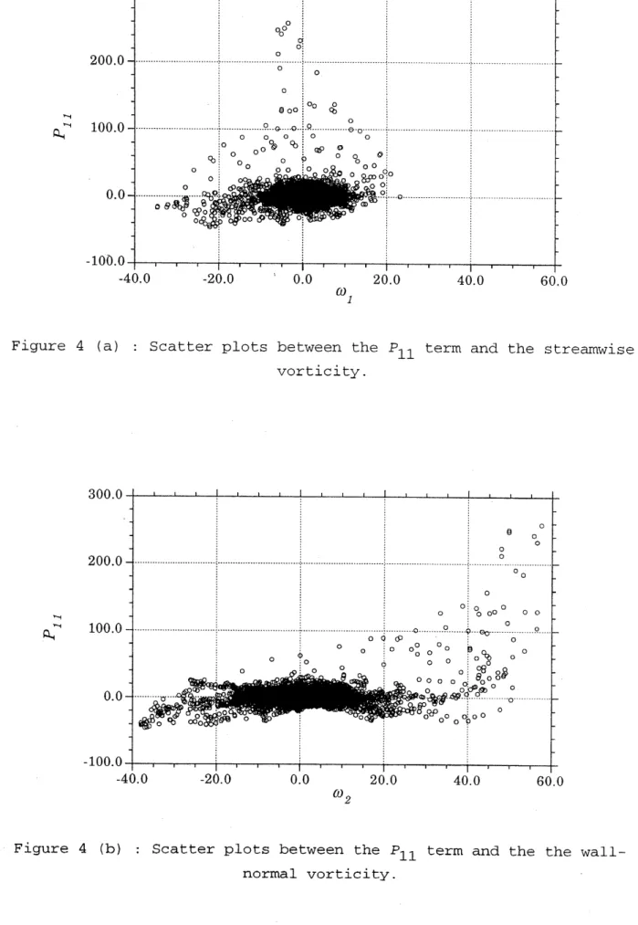
Figures 4 (a) and (b) show thescatter plots between the $P_{11}$ ternl and the strealDwise
and thewall-normal vortices, respectively, which were taken from the region $9\leq y_{+}\leq 21$.
It can be seen in Fig. 4 (a) that large $\overline{\omega}_{1}$ is associated with negative
$P_{\perp\perp}$, whereas large
positive $P_{11}$ generates no significant $\overline{\omega}_{\perp}$. In Fig. 4 (b), large $\overline{\omega}_{\sim}9$ is correlated with large positive $P_{11}$. Thus, principal vortical structures educed in the present
detection are the streamwise vortices generatedalongthe$P_{11}$-Backwardevent and the wall-normal vortices
generated along the $P_{11}$-Forward event.
This result can be explained by using the vortex stretching term in the governing
equation for the grid-scale enstrophy $P_{\omega}=\overline{\omega}_{i}\overline{\omega}_{j}\partial\overline{u}_{i}/\partial x_{j}$. Major term for the streamwise
enstrophy equation is the term $\overline{\omega}_{\perp}\overline{\omega}1\partial\overline{u}_{1}/\partial x_{1}$. It can be readily seen that
$P_{1\perp}$-Backward event provides positive contribution to thisterm, $\mathrm{i}.\mathrm{e}.,$ enhances$\overline{\omega}_{1}$, whereas $P_{1\rfloor}$-Forward event makes negative contribution i.e., reduces $\overline{\omega}_{\perp}$. $\mathrm{S}\mathrm{i}_{1}\mathrm{n}\mathrm{i}\mathrm{l}\mathrm{a}\mathrm{r}\mathrm{l}\mathrm{y}$, the terlll for
the
wall-normal enstrophy equation, $\overline{\omega}_{9}\overline{\omega}_{9}\simarrow\partial\overline{u}_{\underline{9}}/\partial x_{2}$ can be approximates as
$-\overline{\omega}_{-},\overline{\omega}_{2}\partial\overline{u}\perp/\partial.x_{\perp}$. via
the continuity equation. $P_{11}$-Forward event provides positive contribution to this term
and enhances $\overline{\omega}_{2}$, whereas $P_{11}$-Backward event lnakes negative contributioI] i.e., recluces $\overline{\omega}_{2}.12)$
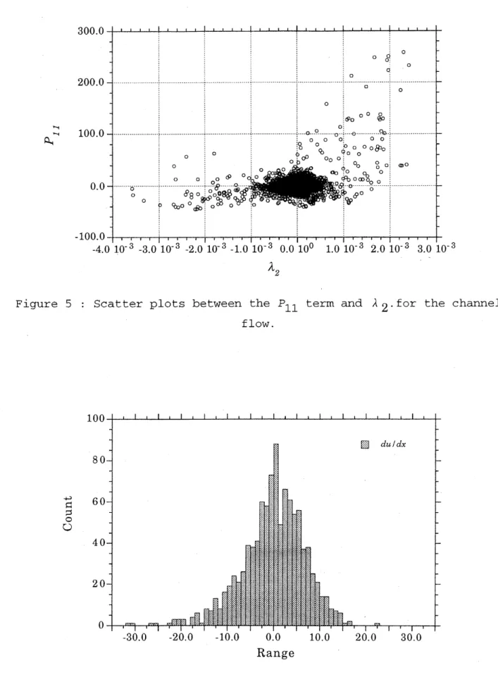
In order to classify the educed vortical structures, we utilized the $\lambda_{2}$ nlethod, where
$\lambda_{2}$ denotes the second largesteigen
value ofthe tensor $s_{ik}s_{\iota_{j}}-+\Omega_{\dot{\mathrm{z}}k}\Omega_{k^{\backslash }j},$$(S_{ij}=(\partial\overline{u}_{i}/oxj+$
$\partial\overline{u}_{j}/\partial x_{i})/2,$$\Omega_{ij}=(\partial\overline{u}_{i}/\partial x_{j}-\partial\overline{u}_{j}/\partial x_{i})/2)$. $11$) Figure 5 shows the scatter plots between
the $P_{11}$ term and $\lambda_{2}$. $P_{11}$-Forward event is primarily correlated with positive
$\lambda_{2}$, while
$P_{\perp\perp}$-Backwardeventis associated with negative
$\lambda_{2}$. That is, the wall-normal vortices
gen-erated with the$P_{11}$-Forwardeventare classified as a vortex sheet, whereas the
streaJuwise
vortices generated with the $P_{11}$-Backward event are classified as a vortex tube.
In summary, forward cascade of the grid-scale energy is associated with the vortex
sheet-like structure, which is consistent with the previous result for the $\mathrm{h}_{\mathrm{o}\mathrm{n})\mathrm{o}\mathrm{g}\mathrm{e}\mathrm{n}}\mathrm{e}\mathrm{o}\mathrm{u}\mathrm{S}$ isotropic turbulence. 13) On the other hand, backward
scatter is associated with the
for-mation of vortex-tube like structure. Figure 6 shows the histogram for the longitudinal velocity derivative $\theta\overline{u}/\partial x$ in the $x-z$ plane at $1/+=12$, obtained fron)
the filtered DNS data. Its distribution is asylnmetric with respect to $\partial\overline{u}/\partial x=0$, and skewed for negative
values. This asymlnetricand non-Gaussian distribution has been noticed, $\mathrm{e}.\mathrm{g}.$, in Vincent
et al. 14) We consider that this occurred so
that the energy cascade beconles forward on
average.
2.2
Energy
transfer
in
mixing
layer and
homogeneous isotropic
turbulence
In this section, we assess the correlation of the energy transfer and $\mathrm{v}\mathrm{o}\mathrm{r}\mathrm{t}\mathrm{e}\mathrm{x}_{-}\mathrm{s}\mathrm{h}\mathrm{e}\mathrm{e}\mathrm{t}/\mathrm{t}\mathrm{u}\mathrm{b}\in 1$
structure in nlixing layer and decaying homogeneous isotropic turbulence.
de-velops in time, and generated DNS data using the $\mathrm{F}_{\mathrm{o}\mathrm{u}\mathrm{r}}\mathrm{i}\mathrm{e}\mathrm{r}/\mathrm{f}\mathrm{i}\mathrm{n}\mathrm{i}\mathrm{t}\mathrm{e}$ difference method, with 192, 128 and 128 grid points, respectively, in the $x,$ $y$ and $\approx$ directions.
6) The Reynolds
nulnber, $Re_{\theta}$, based on the mean velocity difference between the two edges of the lnixing
layer, $\triangle U$, andthe initial momentum thickness, $\theta_{0}$, wasset equal to 200. The
pseudospec-tral Fourier expansion method was used in the $x$ and $z$ directions, whereas the $2\mathrm{n}\mathrm{d}$-order
central finite difference lnethod was used in the $y$ direction. This mixing layer DNS data
was filtered to $96\cross 128\cross 64$ grid points, respectively, in the $x,$ $y$ and $\approx$ directions. As-sessment was done at $t=350,6$) when streamwise rib vortices had been formed in the
braid region between the rollers after the occurrence of a mixing transition, $\perp 5$)
and the flow was in a turbulent regime.
The incompressible homogeneous isotropic turbulence DNS data were generated using the pseudo-spectral method with 128, 128 and 128 grid points, respectively, in the $:\mathrm{r},$ $y$
and $z$ directions. The initial Taylor microscale Reynolds number was approxinlately 100.
Assessment was done using the data when the Taylor microscale Reynolds number was approximately 45. This honlogeneous flow DNS data was filtered to $32\cross 32\mathrm{x}32$ in the
$x,$ $y$ and $z$ directions, respectively.
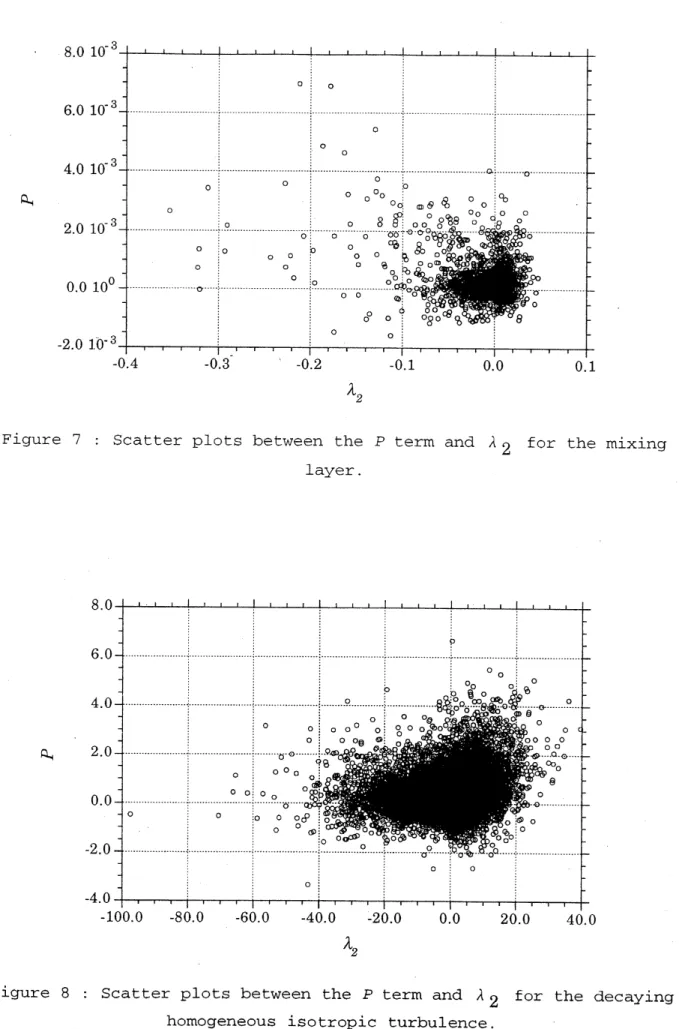
Figures 7 sh$o\mathrm{w}\mathrm{s}$ the scatter plots between the $P$ ternl and
$\lambda_{2}$ obtained for the mixing layer flow. Forward scatter event is rather correlated with negative $\lambda_{2}$, indicating that
energycascade $\mathrm{p}\mathrm{r}\mathrm{i}\mathrm{n}_{\overline{1}}\mathrm{a}\mathrm{r}\mathrm{i}\mathrm{l}\mathrm{y}$occursthrough a tube-like structure, $\mathrm{p}\mathrm{r}\mathrm{e}\mathrm{s}\mathrm{u}\mathrm{n}\overline{\mathrm{l}}$ably by a stretching
of vortex tubes. The degree of an occurrence of the sheet-like structure with positive $\lambda_{2}$
is reduced compared with the result from the channel flow shown in Fig. 5, i.e., the tube-like structure is dominant in the lnixing layer. $\mathrm{S}\mathrm{i}\mathrm{n}\overline{\mathrm{l}}\mathrm{i}\mathrm{l}\mathrm{a}\mathrm{r}$ results were obtained both in the rib region and the braid region of the nlixing layer. This $\mathrm{r}\mathrm{e}\mathrm{l}\mathrm{s}\mathrm{u}1\uparrow J$
nlay be affected by
the low Reynolds nulnber for the DNS data used here. We are currently working on an assessment at the high Reynolds nulnber case using the high ${\rm Re}_{}.\mathrm{v}$nolds nunuber DNS data $(Re_{\theta}=240016))$.
Figures 8 shows the scatter plots between the$P$term and $\lambda_{2}$ obtained for the decaying
homogeneous isotropic turbulence. Overall, the result is similar to that for the channel
flow, i.e., intense forward cascade isprimarily associated with the sheet-like structure and
the degree of an occurrence ofthe sheet-like structure is more enhanced $\mathrm{c}\mathrm{o}\mathrm{n}$)$\mathrm{p}\mathrm{a}\mathrm{r}\mathrm{e}\mathrm{d}$ with the mixing layer. However, it should be noted that the degree of an occurrence of the tube-like structure is not negligibly small compared with the channel flow.
3
Time
development of the
educed
flow
field in the
channel flow
In this section, we pursue the time evolution of the educed flow $\mathrm{n}\mathrm{e}\mathrm{l}\cap \mathrm{d}$ for the channel $\mathrm{f}\mathrm{l}0^{1}\lambda$.
in Section 2. To do this, the effects of the SGS field nlust be correctly represeIlted bv
the SGS models for the SGS stress tensor, $\tau_{ij}$. We have used the $\mathrm{d}\mathrm{y}_{11\mathrm{a}\iota 11}\mathrm{i}_{\mathrm{C}}\cdot \mathrm{t}\mathrm{w}\mathrm{o}-\mathrm{P}\mathrm{a}\mathrm{I}\mathrm{a}\mathrm{I}\mathrm{l}\mathrm{l}\mathrm{e}\mathrm{t}\mathrm{e}\mathrm{r}$
mixed nlodel (DTM $C_{B}-C_{S}$ model 9)$)$ obtained by lineal
$\cdot$ly conlbining the
SGS eddy
viscosity coefficient model (the $\mathrm{s}_{\mathrm{m}}\mathrm{a}\mathrm{g}_{\mathrm{o}\mathrm{r}}\mathrm{i}\mathrm{I}\mathrm{l}\mathrm{s}\mathrm{k}\mathrm{y}$ model 17)$)$ and $\mathrm{s}\mathrm{c}\mathrm{a}\mathrm{l}\mathrm{e}-\sin$)$\mathrm{i}\mathrm{l}\mathrm{a}\mathrm{r}\mathrm{i}\mathrm{t}\mathrm{y}$nlodel
$\perp 8$).
The assesslnent of the previous SGS lllodels, Dynamic Smagorinsky $\mathrm{n}$)$\mathrm{o}\mathrm{d}\mathrm{e}\mathrm{l},$
$19$)
the
dynamic mixed model, 20) the DTM proposed by Salvetti and Banerjee 21) and $C_{B}$’
incompressible $\mathrm{h}_{0111\mathrm{O}}\mathrm{g}\mathrm{e}\mathrm{n}\mathrm{e}\mathrm{o}\mathrm{u}\mathrm{S}$ isotropic turbulence have been previously reported. The
$C_{B}^{l}-C_{S}$ model yielded the most accurate results in both “a priori’ and $‘\iota \mathrm{a}$ posteriori” tests. Particularly important for the present study is the assessment results for the grid
scale-SGS energy transfer. It was found in all of tested cases that the $C_{B}’-C_{S}\mathrm{n}\overline{\perp}\mathrm{o}\mathrm{d}\mathrm{e}\mathrm{l}$
is capable ofaccurate representation of both forward and backward scatters, while other models overestimate forward scatter and underestimate backward scatter. In fact, the
$C_{B}-C_{S}$ model yielded a very accurate approximation for the distribution ofthe $P_{11}$ term
associated with the educed velocity field obtained in Section 2 (figure not shown).
$\mathrm{T}\mathrm{i}\mathrm{n})\mathrm{e}$ evolution of the asymmetric
streakv $\mathrm{s}_{\mathrm{I}}$tructure obtained for $P_{11}$-Forward
event
was pursued in LES using the $C_{B}^{l}-C_{S}$ model. The initial condition was given as the
velocity and pressure fields derived from $P_{1\perp}$-Forward case. With a lapse
of $\mathrm{t}\mathrm{i}_{1}\mathrm{n}\mathrm{e}$, the portion with positive contours catches up with that with negative ones, and the
asynnnet-ric streaky structure in Fig. 2 (a) was transformed into the $\mathrm{s}\mathrm{y}_{\mathrm{l}\mathrm{n}\mathrm{m}\mathrm{e}\mathrm{t}}\mathrm{r}\mathrm{i}\mathrm{C}$ streaky structure. Later, this symmetric structure became asymmetricagain, in which the portion with pos-itive contours were placed $\mathrm{d}\mathrm{o}\mathrm{w}\mathrm{n}\mathrm{s}\mathrm{t}\mathrm{r}\mathrm{e}\mathrm{a}\ln$of that with negative
ones, sinlilar to the contours
shown in Fig. 2 (b) obtained for $P_{11}$-Backward event. Thereby, initially, an intense
for-wardscatter occurred, and torelax this $\mathrm{t}i\mathrm{e}\mathrm{x}\mathrm{c}\mathrm{e},\mathrm{S}\mathrm{s}\mathrm{i}_{\mathrm{V}}\mathrm{e}$” generation
ofthe SGS energy, the flow tended to adjust itself to reduce the cascade. It was found, however, $\mathrm{t}_{}\mathrm{h}\mathrm{a}\mathrm{t}$ the turbulent
state gradually decayed when the educed velocity field wasdirectly used. This was because
a lift-up ofthe low-speed streak was not strong enough to sustain the turbulence. $1^{\underline{)}}$) When the amplitude of turbulent fluctuations was set twice as large as those of the educed velocity field, a lift-up ofthe low-speed streak was initiated. Figure 9 shows the end view of time lines generated in the$x-z$ plane at $y_{+}=12$ for $P_{1\perp}$-Forward case, after
a non-dilllensional time of $1.0tu_{\mathcal{T}}/\delta$ elapsed. The tinle lines for the same plane and at
the same instant obtained for $P_{11}$-Backward case are shown in Fig. 10. The degree of
lift-up of low-speed streak shown in Fig. 9 is much larger than that shown in Fig. 10, implying that more intense lift up occurs in $P_{11}$-Forward event. It was found that this
lift up was caused by a pair of counter-rotating streanlwise vortices located above the
detection point. It should be noted that this lift up did not occur uniformly along the
low speed streak, but it was lnore manifested in the region where the high speed streak
approaches the low speed streak. This result was consistent with that obtained in Fig. 10 that the region with the second largest lift up found in Fig. 10 $(\approx/\delta\simeq 1.0)$ coincided
with the region where the high speed streak approaches the low speed streak. It can be inferred that the largest lift up, or burst, is generated along $P_{11}$-Forward event, leading
to the production of the slllall-scale (SGS) turbulent energy.
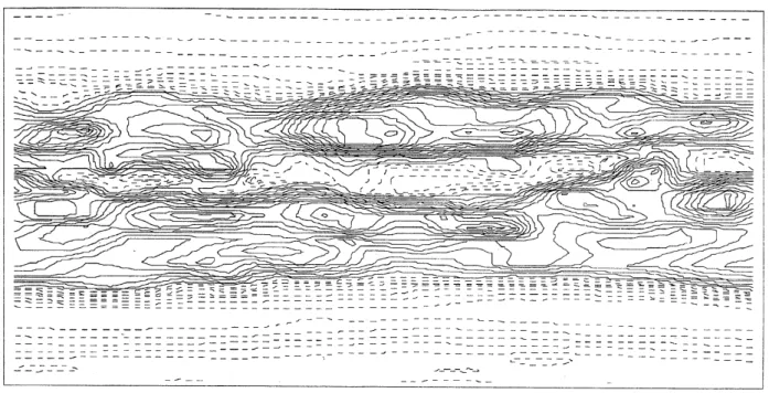
With the lapse oftime, a lift up ofthe low-speed streak intensified and the low-speed streak located in the central region 01 the $x\cdot-z$ plane observed in Fig. 2 (a) was allllost
$\mathrm{P}^{\mathrm{U}\mathrm{n}1}\mathrm{p}\mathrm{e}\mathrm{d}$ out of the sublayer into the buffer laver. Thus,
the wall vicinity became very
tranquil. Figure 11 shows the contours of$\overline{u}’’$ in $\mathrm{t}1_{1}\mathrm{e}.\mathrm{r}-\approx$ plane at
$y_{+}=12$ obtained at
$t=2.2$. The low-speed streak in the central region of the $x-\approx$ plane is $\mathrm{a}\ln\overline{\mathrm{l}}\mathrm{o}\mathrm{s}\mathrm{t}$ invisible, and the central region is mostly occupied with the high-speed fluid. Although another
$1\mathrm{o}\mathrm{v}_{\iota}^{\gamma}$
-speed streak can beseen besides the central region, the$\mathrm{a}\mathrm{n}\mathrm{l}\mathrm{p}\mathrm{l}\mathrm{i}\mathrm{t}\mathrm{u}\mathrm{d}\mathrm{e}$ offluctuations along these streaks is not large enough to cause the lift up. In turn, the down wash (sweep) of
the fluid in the region away from the wall into the near-wall region is initiated. Currently, we consider that this down wash was caused by a large scale streamwise vorticesgenerated
by the G\"ortler type instability. With the injection of the high speed fluid, amplification and destabilization of the low-speed streak found in Fig. 11 occurs, as indicated in the contours of$\overline{u}^{\prime l}$ in the
$x-z$ plane at $y_{+}=12$ obtained at $t=3.8$ shown in Fig. 12, which
leads to the lift up of these low-speed streaks.
We consider thatacyclical repetition of thesethreeprocesses is thescenarioin the
sus-tenance of turbulence for the channel flow. More detailed investigation of these processes
is currently underway.
Acknowledgment
This work was partially supported by the Grant-in-aid, Ministry of $\mathrm{E}\mathrm{d}\mathrm{u}\mathrm{c}\mathrm{a}\mathrm{t}\mathrm{i}_{\mathrm{o}\mathrm{I}1}$, Japan
(No.10650162)
References
1) K. Horiuti, Phys. Fluid,s Al (1989) 426.
2) U. Piomelli, T.A. Zang, C.G. Speziale $\mathrm{a}\mathrm{I}\downarrow \mathrm{d}$ M.Y. Hussaini, Phys. FluidIs
$\underline{\prime}\mathrm{c}2$ (1990)
257.
3) U. Pionlelli, W.H. Cabot, P. Moin and S. Lee, Phys. Fluids A3 (1991) 1766.
4) C. H\"artel, L. Kleiser, U. Friedemann and R. Friedrich, (Phys. Fluids 6 (1994) 3130.
5) K. Horiuti, Phys. Fluids A 5 (1993) 146.
6) K. Horiuti, J. Phys. Soc. Japan 66, 91 (1997).
7) U. Piomelli, Y. Yunfang and R.J. Adrian, Phys. Fluids 8 (1996) 215.
8) P. Moin and J. Kin), J. Fluid Mech. 155 (1985) 441.
9) $\mathrm{I}\backslash \nearrow$. Horiuti, Phys. Fluids 9, 3443 (1997).
$\perp 0)\mathrm{A}.\backslash /^{r}$. Johansson, P.H. Alfredsson and J.
$\mathrm{K}\mathrm{i}\mathrm{n}\overline{\mathrm{l}}$, J. Fluid Mech. 224, 579 (1991).
11) J. Jeong, F. Hussain, W. Schoppa and J. $\mathrm{I}\backslash ^{r}\mathrm{i}\mathrm{m}$, J. Fluid Mech. 332, 185 (1997). 12) W. Schoppa and F. Hussain, Proc. IUTAM Symp. on Dynamics of Slender Vortices
(ed. E. Krause), Aachen, Germany, 183 (1998).
13.) W.T. Ashurst, A.R. Kerstein, R.M. $\mathrm{I}\langle \mathrm{e}\mathrm{r}\mathrm{r}$ and C.H. Gibson, Phys. Fluids 30, 2343
(1987).
14) A. Vincent and M. Meneguzzi, J. Fluid Mech. 225, 1 (1991).
15) M.M. Rogers and R.D. Moser, J. Fluid Mech. 243, 183 (1992).
16) M.M. Rogers and R.D. Moser, Phys. Fluids 6, 903 (1994).
17) J. Smagorinsky, Mon. Weath. Rev. 91, 99 (1963).
18) J. Bardina, Ph.D. dissertation, Stanford UniverSit..V, Stanford, California (1983).
19) M. Germano, U. Piolnelli, P. Moin 811d $1\lambda^{\vee}’.\mathrm{H}$. Cabot, Phys. Fluids A 3, 1760 (1991).
20) Y. Zang, R.L. Street and J. $\mathrm{I}\backslash ^{r}\mathrm{O}\mathrm{S}\mathrm{e}\mathrm{f}\mathrm{f}$, Phys. Fluids A 5, 3186 (1993).
$J_{+}$
Figure 1 : $\mathrm{y}-\mathrm{d}\mathrm{i}\mathrm{S}\mathrm{t}\mathrm{r}\mathrm{i}\mathrm{b}\mathrm{u}\mathrm{t}\mathrm{i}\mathrm{o}\mathrm{n}\mathrm{S}$ for plane-average
of the individual terms in P ノ $P$
$\mathrm{i}\mathrm{i}$ .
Figure 2 (a) : Top view of the contours for streamwise velocity in
the $x-z$ plane at: $y_{+}\sim 12$
.
$\langle$Figure 2 (b) : Top view of the contours for streamwise velocity in
the $\mathit{2}:-Z$ plane at $\mathrm{y}_{+}$ $\sim 12$. ($P_{11}$-Backward event:)
$\eta\frac{\supset}{\alpha}$ $\frac{-^{\mathrm{H}}\vdash}{\mathrm{c}+}$. $\mathrm{a}^{\frac{\mathrm{g}}{\mathrm{o}}}$ $(\mathrm{D}(\mathrm{t}\mathfrak{Q}_{d}\eta$
,
$1rightarrow$ $\omega \mathrm{Z}\mathrm{O}$ $\mathrm{n}_{\dashv}$ $y/\delta$Figure 3 : $\mathrm{y}$ – profiles of the grid-scale turbulence intensities
$\mathrm{o}_{\triangleleft}^{\neg}$
Figure 4 (a) : $\mathrm{S}\mathrm{c}\mathrm{a}\{\mathrm{i}\mathrm{t}\mathrm{i}\mathrm{e}\mathrm{r}$ plots between the
$P_{11}$ $\mathrm{t}:\mathrm{e}\mathrm{r}\mathrm{m}$ and the streamwise
vort:ici$\mathrm{t}\mathrm{y}$.
$\mathrm{Q}_{\backslash }\neg$
Figure 4 (b) : Scatter plots between the $P_{11}$ term and the the
$\mathrm{h}^{\eta}$
Figure 5 : Scatter plots between the $P_{11}$ term and $\lambda_{2}$
.
for the chamelflow.
$\overline{\overline{\mathrm{O}\mathrm{o}}}$
Range
Figure 6 : Histogram for the longitudinal velocity derivative in the
$\mathrm{h}$
$\lambda_{\mathit{2}}$
Figure 7 : Scatter plots between the $P$ term and
$\lambda 2$ for the mixing
layer.
$\mathfrak{Q}_{\neg}$
$\lambda_{\mathit{2}}$
Figure 8 : Scatter plots between the $P$ term and
$\lambda 2$ for the decaying
ら
$z$
Figure 9: End view of $\mathrm{C}$ime lines generated in the
x-z
plane at $y+=12$ $\mathrm{f}$rom
$P11$-Forward cas$\ominus$ a$\mathrm{C}$ $\mathrm{t}$ $\tau/\grave{o}--1.0$
.
ら
$z$
Figure 10 : End view of time lines generated in the
x-z
plane $\mathrm{a}\mathrm{c}$$y+=12$ from $P$ $-\mathrm{B}\mathrm{a}\mathrm{c}\mathrm{k}\mathrm{W}\mathrm{a}\mathrm{r}\mathrm{d}$ case at $\mathrm{C}$ $\tau/\delta=1.0$
.
$———————–\nearrow---\sim---$
$——\sim---’---arrow---’---\vee-’---’--arrow---\vee---\backslash _{----}’---’---\vee---’---’-\sim---’-’--\vee---’-\backslash ---\vee^{--}---\sim---\sim---\sim----\sim---\sim---’---\sim-\wedge---\sim---\sim---\sim---\sim---\sim---$
$—-’——\sim\sim_{arrow}-\sim-$
Figure 11 : Top view of [he $\mathrm{c}\mathrm{o}\mathrm{n}\mathrm{C}\mathrm{o}\mathrm{u}\mathrm{r}\mathrm{s}$ for
$\mathrm{s}\mathrm{C}\mathrm{r}\mathrm{e}\mathrm{a}\mathrm{m}\mathrm{w}\mathrm{i}\mathrm{S}\mathrm{e}\mathrm{v}\mathrm{e}\mathrm{l}_{0}\mathrm{c}\mathrm{i}\mathrm{c}_{Y}$ in the
$x-z$ plane $\mathrm{a}\mathrm{C}\mathrm{y}_{+}\sim$ $12$ and $t=2.2$
Figure 12 : Top view of the $\mathrm{c}\mathrm{o}\mathrm{n}\mathrm{t};\mathrm{o}\mathrm{u}\mathrm{r}\mathrm{S}$ for streamwise velocity in the