修士論文
ケプラー衛星データの系統的解析による長周 期木星型惑星の発見
上原翔
指導教官
:
石崎欣尚首都大学東京大学院 理工学研究科 物理学専攻
2016
年1
月3
目 次
第
1
章 序論3
1.1
太陽系外惑星探査の歴史と長周期惑星. . . . 3
1.1.1
高精度位置観測法(アストロメトリ法) . . . . 5
1.1.2
視線速度法. . . . 6
1.1.3
トランジット法. . . . 7
1.2
ケプラー衛星. . . . 11
1.2.1
軌道. . . . 11
1.2.2
姿勢制御. . . . 12
1.2.3
望遠鏡. . . . 12
1.2.4
焦点面アレイ. . . . 13
1.2.5
時刻系. . . . 14
1.2.6
検出されたイベントの分類. . . . 16
1.3
ケプラーデータに埋もれた長周期惑星の発見. . . . 17
第
2
章 シングルトランジットの同定と軌道周期の推定19 2.1
シングルトランジットの視覚的探索. . . . 19
2.2
シングルトランジットのパラメータ推定. . . . 19
2.2.1
原理. . . . 19
2.2.2
データセットの作成. . . . 20
2.2.3 MCMC
によるトランジットのモデルフィット. . . . 22
第
3
章 シングルトランジットの分類と各系の解説25 3.1
長周期惑星と思われるシングルトランジット. . . . 25
3.1.1 KOI-1096 (KIC 3230491) . . . . 36
3.1.2 KOI-1168 (KIC10460629) . . . . 42
3.1.3 KOI-1174 (KIC 10287723) . . . . 43
3.1.4 KOI-1208 (KIC 3962440) . . . . 46
3.1.5 KOI-1870 (KIC 10187159) . . . . 52
3.1.6 KOI-3349 (KIC 8636333) . . . . 58
3.1.7 KOI-4307 (KIC 3558849) . . . . 61
3.2
各惑星候補のパラメータの統計的性質. . . . 64
3.3
その他に発見された興味深い減光. . . . 64
第
4
章discussion 67 4.1
エキセントリックプラネット候補. . . . 67
4.2
今回発見された惑星候補の特徴. . . . 68
4
4.3
内側の惑星と木星型惑星の間に位置する惑星の観測的欠乏. . . . 68
4.4
コンパクトマルチ系における木星型惑星の存在頻度. . . . 71
1
abstract
2016
年1
月現在、太陽系外惑星の発見数は2000
個を超え、惑星検出を試みながら失敗続きで あった20
年前からは想像もできない進展をみている。惑星系の姿も太陽系と瓜二つの系から、彗星のような楕円軌道の惑星、水星軌道よりも内側に
5
個も惑星が密集する系など非常に多様 であることがわかってきた。惑星検出方法のうち、恒星の前を惑星が通過して影になる現象を観測するトランジット法は、
0.1%程度の減光を検出できればよいのでアマチュアでも容易に惑星の検出が可能である。その
反面、確率の低い事象を観測する制約から、多数の恒星を同時に見張る必要があり、それが太陽 系外惑星発見の黎明期において、当時有力な手法だった視線速度法などと比較して大きな障害 となっていた。しかし、2009
年3
月のケプラー衛星の打ち上げを境に、状況は大きく好転した。ケプラー衛星は主鏡の口径が
1.4 m
であり、地球や太陽が観測に及ぼす影響を避けるために、太陽を中心として地球の後を追いかける太陽周回軌道に投入されている。観測領域ははくちょ う座のごく狭い一角で、一度に
10
万個の恒星を観測することができる。これにより惑星発見数 は1005
個と全体の半数を占めるまでに至った。私は、ケプラー衛星の時系列測光観測データの中に、未確認の木星サイズの惑星候補天体に よるものと考えられる減光
(single transit)
があることを発見した。そこで、ケプラーチームが 真贋問わず惑星候補を1
個以上持っていると認定したKepler Objects of Interest (KOI)
に載っ ている天体7557
個全ての天体のライトカーブに対し視覚的探索を行ったところ、合計28
個のsingle transiting events (STEs)
が存在することを確認した。通常、トランジットが1
回しか観 測できない場合は公転周期を求めることは困難である。私は、既知惑星が1
個以上ある場合に は、それらのパラメータを用いることで未知惑星の公転周期を推定可能であることを理論的に 示した。次に、全ての惑星が既知の多重惑星系のうち、STEと同程度の継続時間と深さのトラ ンジットを起こす惑星を含む系について、敢えて公転周期を未知であると仮定して同時フィット を行い、公転周期推定手法が妥当であることを確認した。既知惑星が1
個以上ある場合はSTE
との同時フィットを、既知惑星無しの場合は主星の密度を与えてフィッティングを行った結果、7
個が海王星サイズから木星サイズの長周期の惑星であり、周期は数年から20
年であると見積 もることができた。またSTE
と内側の惑星との中間付近の公転周期の惑星が欠乏しているよ うに思われたが、シミュレーションの結果、これは観測バイアスに起因するものであることが 判った。さらに、695個の多重惑星系から長周期惑星が5
個見つかった事実から、惑星間の相 対的な軌道傾斜角が小さいと仮定したときに、3 AU以遠のガス惑星は20%以上の確率で存在
していることが判った。このように本研究では、これまで未解明であった長周期の系外惑星を 少なくとも7
個同定し、太陽系と類似した惑星系の形成や構造についての新たな知見を得るこ とができた。3
第
1
章 序論1.1
太陽系外惑星探査の歴史と長周期惑星今日、太陽系外惑星は
2000
個以上が発見され、またその検出手法も多様化・高精度化し、当 初は発見の難しかった太陽系の木星と類似した惑星の発見も少しずつ増えている。表1.1
に各 検出手法の特徴を示す。主星から離れた位置の木星型惑星の存在は、太陽系と同タイプの惑星 系、すなわち内側を岩石を主成分とする地球型惑星が周回している系である可能性を示唆する。このような惑星系の探索は、私達と同じタイプの生命体が他の星の周りの惑星にどれだけ存在 し得るのか、私達はどのようにして生まれたのかという根源的な問いに対する手がかりとして 非常に意義がある。
私達と同じような生命が惑星系内において生存可能な領域、特に惑星表面に海洋を永続的に 維持可能な領域を永続的ハビタブルゾーン
(CHZ)
と呼ぶ。CHZの範囲は、惑星表面の温度、す なわち惑星が受け取る中心星放射の量により決まる。惑星の反射率や大気組成、大気圧が地球 と同じであると仮定すると、CHZと中心星の距離d
∗の古典的な定義は以下の式で与えられる。d
∗=
√ L
∗L
⊙(1.1)
L
∗, L
⊙はそれぞれ恒星、太陽のボロメトリック光度である。太陽の周りの地球のような惑星の 場合、CHZ
の範囲は0.95 - 1.37 AU
の範囲となる([12])。図 1.1
はCHZ
内に入っている可能性の 高い太陽系外惑星の例である。しかし、これらの惑星が地球に似た環境にあるとは、必ずしも 言えない要素がある。Gliese 667C, Gliese 581, HD40307は全て0.7 AU
と、太陽系でいえば金 星ま軌道よりも内側にスーパーアースサイズから海王星サイズの惑星がいくつもひしめき合っ ている惑星系であり、私達の太陽系とはまた異なる姿をしている。その形成過程には惑星の移 動が大きく関わっているとされるが、主星から離れた位置の木星型惑星がなぜ存在しないのか など、依然としてよく分からない点も多い。このように、CHZに入っている惑星は発見されつ つあるものの、内側に地球型惑星、数AU
辺りに木星型惑星という配置の古典的な描像の惑星 系を探すという目標は未だ大きな地位を占めていると云える。代表的な太陽系外惑星の検出方法は、アストロメトリ法、視線速度法、トランジット法、重 力マイクロレンズ法、直接撮像、パルサータイミング法である。表
1.1
に各検出方法の大まか な特徴を示す。ここで太陽系に類似した惑星系を探すにあたり• 1 AU
付近の地球サイズからスーパーアースサイズの惑星の探索•
数AU
付近の木星型惑星の探索という
2
つのアプローチを挙げる。前者は短周期惑星の発見が得意な視線速度法やトランジッ ト法が成果を出しつつある。では後者はどうか。アストロメトリ法は、未だ多くの惑星を検出 する精度には至っていない。重力マイクロレンズ法により検出された惑星は報告が増えてきた4
第1.
序論図
1.1:
ハビタブル惑星の例。縦軸は中心星の質量(M
⊙)、横軸は軌道長半径 (AU)
で、どちらも 対数目盛りである。一番上の恒星が太陽で、比較として地球と火星を右上にプロットしてある。2013
年11
月時点で、Kasting1993
[12
]とはまた異なるCHZ
の範囲の見積もりが使われている(太
陽の周りにおいて内側と外側の境界がそれぞれ0.99 AU, 1.67 AU、緑の領域、 Kopparapu2013)。
Gliese 667Cc, Gliese 581d, g, HD40307g, Kepler-22b
はハビタブルゾーンに入っている可能性が 高いと言われている。http://www.space.com/19522-alien-planet-habitable-zone-definition.html
より引用。が、ある恒星と惑星を持つ恒星が重力レンズ効果による増光を起こすような位置関係になる確 率の比較的高い銀河系中心方向の非常に遠くの恒星の惑星しか見つかっておらず、追観測は事 実上困難である。パルサータイミング法はパルサーの周囲の惑星を発見する手法であるが、超 新星爆発に惑星が耐えられるかどうかについては判っておらず、現在見つかっている惑星につ いても超新星後に後天的に形成された惑星であろうと考えられているため
(ref...)、古典的な所
謂惑星とは厳密には少々定義を異にする。直接撮像では、主星のマスク技術の進歩や、特に地 上観測の場合は補償光学系の進化により、さらなる惑星の発見が期待されている([9], [25])
数十AU
が、数AU
付近の木星型惑星についてはこれからであろう。表
1.1:
各手法の特徴まとめ感度 惑星発見数
アストロメトリ法 長周期・大質量の惑星
1
視線速度法 短周期・大質量の惑星
630
トランジット法 短周期・主星に対し断面積比の大きい惑星
1279
重力マイクロレンズ法 アインシュタインリング付近( ∼ 2.5 AU)
の離角の惑星43
直接撮像 年齢が若く高温で大質量であり、離角の大きい惑星
64
パルサータイミング法 長周期・大質量の惑星
23
残る視線速度法とトランジット法はどちらも短周期の惑星に感度があり、一見木星類似惑星 の検出には不向きであるように思われる。しかし、長期間の観測により、徐々に長周期惑星も 発見され始めている。視線速度法の精度は
1ms
−1と、地球による太陽のふらつきを検出できる ところにまで達し、木星類似惑星に手が届きつつある([2], [16], [1])。
状況はトランジット法についても同様であるが、視線速度法には無い利点として、以下の
2
点を挙げることができる。1.1.
太陽系外惑星探査の歴史と長周期惑星5 M. Bedell et al.: The Solar Twin Planet Search. II.
Table 1. Best-fit parameters and uncertainties for HIP11915b.
Parameter Value Uncertainty
P [days] 3830 150
K [m s
1] 12.9 0.8
e 0.10 0.07
! + M
0[rad] 3.0 1.3
! - M
0[rad] 2.4 0.1
↵ [m s
1(unit S
HK)
1] 160 60
C [m s
1] –11.0 1.3
J
[m s
1] 1.8 0.4
m
psin(i) [M
Jup] 0.99 0.06
1a [AU] 4.8 0.1
1RMS [m s
1] 2.9
Notes.
(1)Error estimates do not include uncertainties on the stellar pa- rameters, which were taken from Ramírez et al. (2014).
value from RV, S
HK, BIS, and FWHM for simplicity. This means that the o ↵ set parameter C is partially set by the di ↵ erence be- tween the median RV of the data set and the systemic RV of the star, but also includes the RV o↵set in the linear fit with the median-subtracted S
HKvalues (or any other correlations used in the model; see Sect. 3.2).
All of the fit parameters were given uniform priors except for P and K, which were sampled in log-space with a log- uniform prior. We ran five parallel chains and used the require- ment of a Gelman-Rubin test statistic below 1.01 for all pa- rameters to avoid non-convergence (Gelman & Rubin 1992).
The best-fit orbital solution, plotted in Fig. 1, corresponds to an approximately Jupiter-mass planet on a 10-year orbit with eccentricity consistent with zero (see Table 1). As seen in the MCMC posterior distributions (Fig. 5), the chief source of un- certainty in the period measurement is in its degeneracy with eccentricity and the associated argument of periapse, parame- ters that are inevitably poorly constrained when only one orbit has been observed. The best-fit jitter term is consistent with the predicted stellar jitter of 2.1 m s
1from the formula of Wright (2005).
After subtracting the best-fit planet signal, we searched for additional signals in the residuals with a generalized Lomb- Scargle periodogram analysis (Zechmeister & Kürster 2009).
No significant periodicities were identified in the residuals to the planet fit or in the residuals to the planet and the fitted S
HKtrend. We place constraints on the presence of additional planets in the system using a test based on the bootstrapping and injec- tion of a planet signal into the residuals. For this test, we use the residuals to the planet fit only, and inflate the error bars (with jitter included) such that a flat-line fit to the residuals gives a re- duced chi-squared of one. We then run a set of trials in which the RV data are resampled with replacement at the times of ob- servation, a planet signal with period and semi-amplitude fixed and the other orbital parameters randomized is injected, and the reduced chi-squared of a flat-line fit to these simulated data is measured. If the chi-squared statistic has increased with three- sigma significance in 99 out of 100 trials at a given period and velocity semi-amplitude, we consider such a planet signal to be excluded based on its inconsistency with the scatter in the actual RVs. We run this trial until upper limits on planet presence are found for all of the periods in a log-sampled grid. The results rule out the presence of gas giants within a 1000-day orbital period, leaving open the possibility of inner terrestrial planets (Fig. 2).
Fig. 1. Best-fit orbital solution for HIP11915b. Data points are the ob- served RVs with o↵set and S
HKcorrelation terms subtracted. One resid- ual point is located outside of the plot range, as denoted by the arrow.
Fig. 2. Exclusion limits on potential planets in the RV data after sub- traction of the Keplerian signal. Any signal in the parameter space located above the lines plotted would have induced a larger scatter in the RV residuals with three-sigma significance if present. Potential trends with activity indicators were not removed for this test to avoid underestimating the RV scatter.
3.2. Alternative model choices
It is not obvious from theory that the Keplerian + S
HKcorrela- tion model used above should be the best model choice. Other activity indicators exist and have been used with success to re- move activity trends from RVs in the past. Chief among these are BIS and FWHM, both characteristics derived from the RV cross- correlation function (CCF) which measure the average spectral line asymmetry and / or broadening at the epoch of the observa- tion (see, e.g., Queloz et al. 2001, 2009). Either BIS or FWHM could potentially be used in place of S
HK. Also, because these in- dicators arise from distortions to the rotationally broadened stel- lar absorption lines while S
HKprobes chromospheric emission, we could combine S
HKwith a CCF-derived measurement to si- multaneously track two separate physical indicators of activity.
We considered several alternative models before settling on the Keplerian + S
HKmodel as the best choice. A summary of the models tried is given in Table 2. In all cases, the fitting was done with an MCMC as described above. The inclusion of a Keplerian signal is strongly justified, with the Keplerian + S
HKfit having a false alarm probability on the order of 10
15compared to the best fitting activity model (S
HK+ FWHM). While the lowest
2A34, page 3 of 8
図
1.2:
視線速度法で発見されたHIP11915b。質量の下限値 0.99M
jで、公転周期は3830
日。•
あくまで断面積の大きい惑星に感度があるのであり、惑星半径が大きい必要は無い。•
トランジットの検出さえできれば(主星に対し惑星半径が大きければ)、公転周期によら
ず検出は可能である。言わば、数を打てば地球類似惑星も木星類似惑星も検出可能なのである。そのためには多数の 恒星を同時に長期間見張り続け、トランジットの検出確率を上げる必要があるが、他の手法よ りも導入が簡単であることから、アマチュア天文家を含め世界中で観測が行われている。後述 のケプラー衛星の観測も併せ、太陽系に類似した惑星系の発見の素地は整っていると云える。
そこで、私は長周期の木星型惑星の発見手法としてトランジット法を選択した。以下では、太 陽系外惑星の発見の歴史と、歴史的に使われてきたアストロメトリ法
(1.1.1
節)、視線速度法(1.1.2
節)、トランジット法(1.1.3
節)について概説する。また、2009年の打ち上げから1000
個 以上のトランジット惑星を発見しており、私が惑星の検出にそのデータを用いたケプラー衛星 についても(1.2
節) 今日のように2000
個を超す太陽系外惑星を発見できるようになるまでの道 のりは、決して平坦なものではなかった。16
世紀、ジョルダーノ・ブルーノは太陽以外の星の周りの惑星系の存在を初めて提唱した。当時は地動説が出てきたばかりで未だ天動説が主流であり、地動説をもとにした彼の説は異端 との誹りを受けることとなった。人類が太陽系外惑星の存在を常識と考えるようになったのは、
17
世紀にケプラーの法則が発見されてからさらに後、20世紀になってからであった。1.1.1
高精度位置観測法(
アストロメトリ法)
太陽系外惑星の探索はアストロメトリ法から始まった。主星の周りを惑星が公転していると、
主星も同じ周期でわずかにふらつく。このふらつきを天球面上での動きとして捉えるのがアス トロメトリ法である。質量
m
∗の主星の周りを質量m
pの惑星が距離a
だけ離れて公転している6
第1.
序論 とき、距離d
においてアストロメトリ法により観測されるシグナルの大きさθ
はθ = m
pm
∗a d =
( G 4π
2)
1/3m
pm
2/3∗P
2/3d
= 3[µas] m
pm
⊕( m
∗m
⊙)
−2/3( P yr
)
2/3( d pc
)
−1(1.2)
で与えられる。式
(1.2)
から、質量の大きく公転周期の長い惑星の検出が容易であることがわか る。当時ホットジュピターのように主星に近接した木星型惑星の存在は知られておらず、惑星 系は太陽系と同様に地球型惑星が系の内側に密集し、外側に木星型惑星が配置しているであろ うという先入観があった。また、アストロメトリ法は不可視伴星の検出実績(シリウス B
など) が既にあったのに対し、同様に主星のふらつきから惑星の検出を行う視線速度法(後述)
は主星 のごく近傍の伴星の方が検出し易いことから、アストロメトリ法の選択は最も主星をふらつか せるであろう太陽系の木星と類似した惑星を探すという目的に適っているといえた。1960年代 には、バーナード星に周期24
年、木星の半分の質量を持つ惑星の存在が報告された。しかし、当時アストロメトリ法の精度は悪く、10pc離れた位置から太陽を観測した時の木星に起因する
ふらつき
( ∼ 0.5[mas])
さえ捉えることはできなかった。バーナード星の惑星と思われたシグナルも望遠鏡の誤差であると片付けられてしまい、今日に至るまで長らく日の目を見ることは無 かった。
アストロメトリ法の長所としては、上述の通り長周期惑星に感度がある点、位置観測のみを 行うため主星の種類を問わない点が挙げられる。さらに、惑星の軌道面の傾きに依らないため、
惑星の真の質量を決定することができる点は他の手法には無い利点である。視線速度法では短 周期の惑星が発見し易く、また主星が明るくなければ高精度の観測が困難となるなど、アスト ロメトリ法は視線速度法と相補的な関係にあるといえる。将来の更なる位置観測精度向上に加 え、地球大気の揺らぎの影響を受けない宇宙空間からの観測により、視線速度法やトランジッ ト法での発見が難しい長周期惑星の発見が期待される。
1.1.2
視線速度法視線速度法は、アストロメトリ法とは異なり主星のふらつきの観測者から見た視線方向成分 を観測し、間接的に惑星の存在を推定する手法である。質量
m
p、離心率e
の惑星を持つ質量m
∗の恒星の視線速度の平均値K
は次のように書くことができる。K = 28.4329[ms
−1]
√ 1 − e
2m
psin i m
j( m
∗+ m
pm
⊙)
−2/3( P yr
)
−1/3(1.3)
主星が観測者に対し近づく場合、ドップラー効果により主星の光の波長が短い方にずれ、逆 に観測者から遠ざかる場合は波長が長い方にずれる。一方、barycentric系においてドップラー 効果により元の波長
λ
0から変化した値の平均値をλ
Bとすると、光速をc
として主星の視線速 度の平均値はK = c λ
B− λ
0λ
0(1.4)
λ
B= λ
obs(
1 + 1
c k · v
obs)
[ms
−1] (1.5)
1.1.
太陽系外惑星探査の歴史と長周期惑星7
となる。連星系の場合は相対論的効果を無視できないが、惑星による主星のふらつきは小さい ものとして非相対論的取り扱いを行っている。式(1.3), (1.4), (1.5)
より、主星の視線速度の観 測から惑星の質量を、視線速度の時系列変化の形状から離心率を、変動周期から公転周期を求 めることができる。また、式(1.3)
から惑星の質量が大きいほど、公転周期が短いほど検出が容 易であることがわかる。ただし我々が観測しているのは主星のふらつきを我々の視線方向に射 影した成分なので、実際に得られる観測量はm
psin i
であり、惑星質量の下限値のみが判るこ とに注意を要する。主星の光のドップラー変位は、高分散分光して得られるスペクトル線の位置の変化として測 定される。仮に太陽系の木星を視線速度法で検出しようとすると、木星が太陽を揺らすときの 速度の振幅は
12.4ms
−1であり、可視域(550nm)
の波長変化にして2.0 × 10
−4nm
に相当し、こ の微小なスペクトル線の移動を測定しなければならないが、通常の分光観測では分光器の微小 な温度変化や伸縮により測定精度は数100ms
−1となってしまい、木星の検出はできなくなって しまう。そこで、吸収線の位置がよく判っているガスを封入したガス吸収セルに恒星の光を通 して分光するという手法が用いられる。こうすることで、恒星のスペクトルにガスの吸収線が 分光器の状態をも反映した時々刻々の物差しとして重なり、機器的な誤差を除いた分光観測を 行うことができる。現在広く用いられているヨウ素ガスは500-620nm
に無数の細い吸収線を持 ち、太陽型星の可視光観測に適している。1980
年代までにはこの手法により視線速度法の精度は10ms
−1までに向上し、木星類似惑星 の検出は秒読みかと思われた。しかしながら、ここでも”木星類似惑星”の検出という目的が仇 となり、足下に転がっていたより短周期の木星型惑星という当時としては考えられないような 惑星の発見はできなかった。また、カナダのチームは上述のガスセル法を用いた視線速度法で12
年間かけて21
個の恒星を観測し惑星の存在を否定するという結論に至ったが、現在の惑星検出確率
5%を考えると、当時は観測天体の少なさや不運も重なって見逃しの連続となってし
まった面も否めない。
1995
年10
月、スイスのMichel Mayor
とDidier Queloz
のチームはペガサス座51
番星に公転 周期4
日、木星の半分の質量を持つ惑星を視線速度法により発見した[18]。この惑星が主星を
揺らす速度の振幅は70ms
−1であり、十分に検出が可能であった。これを契機に先入観が崩壊 し、見逃され続けてきた短周期惑星の発見ラッシュが始まるとともに、惑星の移動を含めた惑 星系の形成理論の大幅な見直しが為された。1.1.3
トランジット法一方でこの数年で大きく台頭したのが、恒星の前面を惑星が通過し影になる様子を捉えるこ とで惑星の検出を行うトランジット法である。トランジットの幾何学的構造を図
1.3
に示す。トランジット法では、惑星の通過に伴う減光が大きければ大きい程検出が容易になる。惑星 からの放射は一定であるとし、トランジットをトラペゾイドで近似すると、トランジット時の 減光の深さ
δ
はδ ≈ k
2[
1 − I
p(t
0) I
∗]
(1.6)
k = R
pR
∗(1.7)
8
第1.
序論Fig. 2.— Illustration of a transit, showing the coordinate system discussed in Section 2.1, the four contact points and the quantitiesT andτdefined in Section 2.3, and the idealized light curve discussed in Section 2.4.
(R⋆+Rp)/rwhereris the instantaneous star-planet dis- tance. This cone is called thepenumbra. There is also an in- terior cone, theantumbra, defined bysinΘ= (R⋆−Rp)/r, inside of which the transits are full (non-grazing).
A common situation is thateandωare known andiis unknown, as when a planet is discovered via the Doppler method (see chapter by Lovis and Fischer) but no informa- tion is available about eclipses. With reference to Figure 3, the observer’s celestial longitude is specified byω, but the latitude is unknown. The transit probability is calculated as the shadowed fraction of the line of longitude, or more sim- ply from the requirement|b|<1 +k, using equations (7-8) and the knowledge thatcosiis uniformly distributed for a randomly-placed observer. Similar logic applies to occulta- tions, leading to the results
ptra =
!R⋆±Rp
a
" !1 +esinω 1−e2
"
, (9)
pocc =
!R⋆±Rp
a
" !1−esinω 1−e2
"
, (10) where the “+” sign allows grazing eclipses and the “−” sign excludes them. It is worth committing to memory the results for the limiting caseRp≪R⋆ande= 0:
ptra=pocc=R⋆
a ≈0.005
!R⋆
R⊙
"# a 1 AU
$−1
. (11)
For a circular orbit, transits and occultations always go to- gether, but for an eccentric orbit it is possible to see transits without occultations or vice versa.
In other situations, one may want to marginalize over all possible values ofω, as when forecasting the expected number of transiting planets to be found in a survey (see Section 4.1) or other statistical calculations. Here, one can calculate the solid angle of the entire shadow band and di- vide by4π, or average equations (9-10) overω, giving
ptra=pocc=
!R⋆±Rp
a
" ! 1 1−e2
"
. (12) Suppose you want to find a transiting planet at a particu- lar orbital distance around a star of a given radius. If a frac- tionηof stars have such planets, you must search at least N ≈(ηptra)−1stars before expecting to find a transiting planet. A sample of>200η−1Sun-like stars is needed to find a transiting planet at 1 AU. Close-in giant planets have an orbital distance of approximately 0.05 AU andη≈0.01, givingN >103stars. In practice, many other factors affect the survey requirements, such as measurement precision, time sampling, and the need for spectroscopic follow-up observations (see Section 4.1).
2.3 Duration of eclipses
In a non-grazing eclipse, the stellar and planetary disks 3
図
1.3:
トランジットの幾何学的構造I
∗, I
pはそれぞれ主星及び惑星の放射、t0はトランジット中心時刻を表す。Ip≪ I
∗ と近似す るとδ ≈ k
2(1.8)
と記述することができる。式
(1.8)
より、惑星が主星と比較して相対的に大きければδ
が大きく なることがわかる。inpact parameter b
は、観測者から見て主星面に惑星を投影したときの、主星中心からの惑星中心の距離を主星の半径
R
∗で規格化したものである。b = a
R
∗cos i (1.9)
i
は軌道傾斜角であり、観測者の視線方向と軌道面が垂直な位置関係のときをi = 0 deg
とし、そこからのずれを計量する。
惑星の縁が主星面内に少しでも入ればトランジットは必ず起きる。従って、トランジットが 起きる条件は
| b | < 1 + k
となり、トランジットが起きる確率p
tra
はp
tra=
( R
∗± R
pa
) ( 1 + e sin ω 1 − e
2)
(1.10)
と書ける。
R
∗, R
pはそれぞれ主星及び惑星の半径、aは軌道長半径、eは離心率、ωは近点の位 相である。また、”-”は通常のトランジット、 ”+”は主星の縁をかすめるように通過する grazing transit
を指す。Rp≪ R
∗、e= 0
と近似するとp
tra= R
∗a (1.11)
と記述できる。ωで
marginalize
すると、p
tra=
( R
∗± R
pa
) ( 1 1 − e
2)
(1.12)
1.1.
太陽系外惑星探査の歴史と長周期惑星9
Fig. 3.— Calculation of the transit probability. Left.—Transits are visible by observers within the penumbra of the planet, a cone with opening angle Θ with sin Θ = (R
⋆+R
p)/r, where r is the instantaneous star-planet distance. Right.—Close-up showing the penumbra (thick lines) as well as the antumbra (thin lines) within which the transits are full, as opposed to grazing.
are tangent at four contact times t
I–t
IV, illustrated in Fig- ure 2. (In a grazing eclipse, second and third contact do not occur.) The total duration is T
tot= t
IV− t
I, the full duration is T
full= t
III− t
II, the ingress duration is τ
ing= t
II− t
I, and the egress duration is τ
egr= t
IV− t
III. Given a set of orbital parameters, the various eclipse du- rations can be calculated by setting equation (5) equal to R
⋆± R
pto find the true anomaly at the times of contact, and then integrating equation (44) of the chapter by Murray and Correia, e.g.,
t
III− t
II= P 2π √
1 − e
2!
fIIIfII
"
r(f) a
#
2df. (13) For a circular orbit, some useful results are
T
tot≡ t
IV− t
I= P π sin
−1$ R
⋆a
% (1 + k)
2− b
2sin i
&
, (14)
T
full≡ t
III− t
II= P π sin
−1$ R
⋆a
% (1 − k)
2− b
2sin i
&
. (15) For eccentric orbits, good approximations are obtained by multiplying equations (14-15) by
X(f ˙
c) [e = 0]
X(f ˙
c) =
√ 1 − e
21 ± e sin ω , (16) a dimensionless factor to account for the altered speed of the planet at conjunction. Here, “+” refers to transits and
“ − ” to occultations. One must also compute b using the eccentricity-dependent equations (7-8).
For an eccentric orbit, τ
ingand τ
egrare generally unequal because the projected speed of the planet varies between
ingress and egress. In practice the difference is slight; to leading order in R
⋆/a and e,
τ
e− τ
iτ
e+ τ
i∼ e cos ω ' R
⋆a (
3) 1 − b
2*
3/2, (17) which is <10
−2e for a close-in planet with R
⋆/a = 0.2, and even smaller for more distant planets. For this reason we will use a single symbol τ to represent either the ingress or egress duration. Another important timescale is T ≡ T
tot− τ , the interval between the halfway points of ingress and egress (sometimes referred to as contact times 1.5 and 3.5).
In the limits e → 0, R
p≪ R
⋆≪ a, and b ≪ 1 − k (which excludes near-grazing events), the results are greatly simplified:
T ≈ T
0% 1 − b
2, τ ≈ T
ok
√ 1 − b
2, (18) where T
0is the characteristic time scale
T
0≡ R
⋆P
πa ≈ 13 hr ' P
1 yr (
1/3'
ρ
⋆ρ
⊙(
−1/3. (19) For eccentric orbits, the additional factor given by equa- tion (16) should be applied. Note that in deriving equa- tion (19), we used Kepler’s third law and the approximation M
p≪ M
⋆to rewrite the expression in terms of the stel- lar mean density ρ
⋆. This is a hint that eclipse observations give a direct measure of ρ
⋆, a point that is made more ex- plicit in Section 3.1.
2.4 Loss of light during eclipses
The combined flux F (t) of a planet and star is plotted in Figure 1. During a transit, the flux drops because the 4
Fig. 3.— Calculation of the transit probability. Left.—Transits are visible by observers within the penumbra of the planet, a cone with opening angle Θ with sin Θ = (R
⋆+ R
p)/r, where r is the instantaneous star-planet distance. Right.—Close-up showing the penumbra (thick lines) as well as the antumbra (thin lines) within which the transits are full, as opposed to grazing.
are tangent at four contact times t
I–t
IV, illustrated in Fig- ure 2. (In a grazing eclipse, second and third contact do not occur.) The total duration is T
tot= t
IV− t
I, the full duration is T
full= t
III− t
II, the ingress duration is τ
ing= t
II− t
I, and the egress duration is τ
egr= t
IV− t
III. Given a set of orbital parameters, the various eclipse du- rations can be calculated by setting equation (5) equal to R
⋆± R
pto find the true anomaly at the times of contact, and then integrating equation (44) of the chapter by Murray and Correia, e.g.,
t
III− t
II= P 2π √
1 − e
2!
fIIIfII
"
r(f ) a
#
2df. (13) For a circular orbit, some useful results are
T
tot≡ t
IV− t
I= P π sin
−1$ R
⋆a
% (1 + k)
2− b
2sin i
&
, (14)
T
full≡ t
III− t
II= P π sin
−1$ R
⋆a
% (1 − k)
2− b
2sin i
&
. (15) For eccentric orbits, good approximations are obtained by multiplying equations (14-15) by
X ˙ (f
c) [e = 0]
X ˙ (f
c) =
√ 1 − e
21 ± e sin ω , (16) a dimensionless factor to account for the altered speed of the planet at conjunction. Here, “+” refers to transits and
“ − ” to occultations. One must also compute b using the eccentricity-dependent equations (7-8).
For an eccentric orbit, τ
ingand τ
egrare generally unequal because the projected speed of the planet varies between
ingress and egress. In practice the difference is slight; to leading order in R
⋆/a and e,
τ
e− τ
iτ
e+ τ
i∼ e cos ω ' R
⋆a (
3) 1 − b
2*
3/2, (17) which is <10
−2e for a close-in planet with R
⋆/a = 0.2, and even smaller for more distant planets. For this reason we will use a single symbol τ to represent either the ingress or egress duration. Another important timescale is T ≡ T
tot− τ , the interval between the halfway points of ingress and egress (sometimes referred to as contact times 1.5 and 3.5).
In the limits e → 0, R
p≪ R
⋆≪ a, and b ≪ 1 − k (which excludes near-grazing events), the results are greatly simplified:
T ≈ T
0% 1 − b
2, τ ≈ T
ok
√ 1 − b
2, (18) where T
0is the characteristic time scale
T
0≡ R
⋆P
πa ≈ 13 hr ' P
1 yr (
1/3'
ρ
⋆ρ
⊙(
−1/3. (19) For eccentric orbits, the additional factor given by equa- tion (16) should be applied. Note that in deriving equa- tion (19), we used Kepler’s third law and the approximation M
p≪ M
⋆to rewrite the expression in terms of the stel- lar mean density ρ
⋆. This is a hint that eclipse observations give a direct measure of ρ
⋆, a point that is made more ex- plicit in Section 3.1.
2.4 Loss of light during eclipses
The combined flux F (t) of a planet and star is plotted in Figure 1. During a transit, the flux drops because the 4
図
1.4:
トランジットが観測できる領域ここで、ある半径の主星の周りのある軌道半径にある惑星を検出することを考える。そのよ うな惑星が割合
η
で存在しているとき、トランジットを見つけるためには観測者は最低でもN ≈ (ηp
tra)
−1個の恒星をサーベイする必要がある。例えば1AU
の位置にある太陽型星周りの 惑星の場合、200η−1個以上の恒星を見張ることになる。0.05AUと非常に近接した惑星が1%の
確率で存在しているときは、1000個に1
個の割合でトランジットが観測できるだろう。トランジット法で惑星を探索するとき、既に惑星が存在することが判っている系でトランジッ トが起きるかどうか確認するか、或は非常に多くの恒星をサーベイして惑星のトランジットを 探すかの
2
通りの方針が考えられる。歴史的にトランジット法は視線速度法の後を追う形で発 展したため、まずは前者の方針でトランジット惑星の探索が行われた。最初の探索では64
個の 既知の系に6
個のトランジット惑星が発見された([3], [10], [19])。このときトランジットを起こ
す確率は式(1.10)
で与えられる。次に、サーベイによりトランジット惑星を検出するときのシグナルの要求水準を考えてみる。
先ほど議論したように、0.05AUの位置の惑星のトランジットを検出するためには太陽型星を
1000
個以上サーベイする必要がある。観測的には、1%の減光を捉えること、さらに3
日( ∼ P )
以上の継続的観測が要請される。理想的な条件の近傍の恒星の観測に際しての制限が光子揺ら ぎのみであるとき、トランジットに対する感度はR
6p/P
5/3で与えられる([8])。
このように、測光観測は視線速度法と併せた探索と比較して効率が悪い。しかしながら、視 線速度法には大きな望遠鏡や複雑な分光装置が要求されるのに対し、測光観測は口径
10cm
の 望遠鏡さえあれば十分に1%
の減光を検出し得るという手軽さが利点である。従って、多くの 天文学者がこぞって測光観測に注力し、10を超すサーベイが行われた。毎月
10
個から100
個のホットジュピターが発見されるとの予想もあったが、2
つの障害が立ち ふさがり、惑星発見数のボトルネックとなった。その1
つは高頻度で見つかる食連星であった。連星の相互食が直接受かるものや、不可視伴星の明るさにより本来非常に深いはずの連星によ る減光が過小評価される系などがあり、特に後者は減光が惑星サイズにまでなると惑星との判 別が困難を極めた。あるサーベイではこれら”false positive”の数が惑星候補の
10
倍に上った。もう
1
つの障害は相関ノイズである。多くのライトカーブが都合良くきれいなはずもなく、こぶ やくぼみ、脈動などがトランジットの検出の邪魔となる。これらはCCD
の感度ムラや、恒星表 面の活動など多様な原因により表れる。これらの障害をうまく克服できたのは少数のチームだっ たが、OGLEチームは口径1m
の望遠鏡で14-16
等級の恒星を、TrES, XO, HAT, SuperWASP10
第1.
序論 の各チームは口径0.1m
の望遠鏡で10-12
等級の恒星をそれぞれサーベイし、多数のトランジッ ト惑星を発見した。以上の問題をうまく排除してなお、地上からの観測である限りは地球大気の揺らぎや昼夜サ イクル、天候の影響からは逃れることはできない。そこで打ち上げられたのが
CoRoT
とケプ ラー衛星である。1.2節ではケプラー衛星について詳説する。1.2.
ケプラー衛星11
1.2
ケプラー衛星ケプラー衛星は、トランジット法により銀河系内において地球サイズの惑星やハビタブル ゾーンに位置する惑星の探索を目的として
2009
年3
月6
日に打ち上げられた、1.4mの反射鏡と
0.95m
のレンズを持つシュミット式の反射屈折望遠鏡である。シュミット式望遠鏡としてはこれまでに作られた中で
9
番目の大きさであり、地球周回軌道の外側に投入されたものとして は最大である。当初のミッション期間は3.5-6
年を想定していた。Kepler: NASA’s First Mission Capable of Finding Earth-Size Planets
National Aeronautics and Space Administration
PRESS KIT/FEBRUARY 2009
www.nasa.gov
図
1.5:
ケプラー衛星の観測の想像図表
1.2:
ケプラー衛星の概要 観測軌道Earth-trailing heliocentric
公転周期371
日外形寸法 高さ
4.7m
衛星質量
1052.4kg
発生電力
1100W
打ち上げ
2009
年3
月5
日10
時48
分(EST)
ミッション期間3.5 - 6
年1.2.1
軌道ケプラー衛星の軌道は太陽を中心としており、周期
371
日で地球を追いかけるように運動している
(図 1.7)。この軌道において衛星はゆっくりと地球から遠ざかり、3.5
年が経過した時点で地球からの距離は
0.5AU
となる。この軌道のメリットは、非常に安定してある一方向を向か12
第1.
序論表
1.3:
ケプラー衛星の基本仕様口径
2.7 m
視野面積
105 deg
2CCD
枚数42 array
CCD
サイズ59 × 28 mm
ピクセル数
2200 × 1024
観測帯域(FWHM) 435 to 845 nm
暴露時間
6.019802903 sec
読み出し時間0.5189485261 sec
Kepler: NASA’s First Mission Capable of Finding Earth-Size Planets Press Kit
Spacecraft
Like all spacecraft, Kepler’s design is a delicate balance of form and function. The form is the spacecraft’s dimensions and weight, dictated by the size and power of the launch vehicle lifting it into space. The function is the instrument observing capabilities of the scientific cargo onboard the spacecraft.
As the spacecraft instrument is tasked to survey many stars to determine the prevalence of Earth-size planets, the spacecraft exists to serve its one instrument – a photometer designed to measure the brightness variations of stellar targets as planets cross in front of them. The spacecraft provides the power, pointing, commanding, data storage and data transmission for the photometer. The photometer itself contains the largest camera NASA has launched into space. The spacecraft includes two command and control computers, a solid state data recorder, Ka-band and X-band communication systems, two star trackers, reaction wheels and a reaction control system.
The spacecraft attitude is three-axis stabilized using a line-of-sight pointing control system. The electrical power distribution subsystem uses direct energy transfer, with a fixed solar array and a Li-Ion battery. A fixed solar array minimizes jitter disturbances and shades the photometer. The spacecraft bus structure is fabricated from aluminum honeycomb. A body-mounted high-gain antenna is used for high-rate data transmission. Two omni-directional low-gain antennas are used for low-rate data transmission and commanding.
Pointing at a single group of stars for the entire mission greatly increases the thermal and hence photometric stability and simplifies the spacecraft design. Other than the small reaction wheels used to maintain the pointing and an ejectable cover, there are no other moving or deployable parts onboard Kepler. The only liquid is a small amount of hydrazine
for the thrusters, which is kept from sloshing by a pressurized membrane. This design enhances the pointing stability and the overall reliability of the spacecraft.
Spacecraft Structures and Mechanisms
The majority of Kepler’s systems and subsystems are mounted on a low-profile hexagonal box which is wrapped around the base of the photometer. The hexagonal box structure consists of six shear panels, a top deck, bottom deck, reaction control system deck, and the launch vehicle adapter ring. Construction of the shear panels, decks, and solar array substrates, consists of sandwiched aluminum face-sheets on an aluminum honeycomb core. The six shear panels provide structure to accommodate mounting of the spacecraft electronics, portions of the photometer electronics, battery, star trackers, reaction wheels, inertial measurement units, radio equipment, and high- and low-gain antennas.
The top deck shear panel provides the mounting surface for the solar array panels. The bottom deck provides the interface to the photometer and also supports
the thrusters, associated propellant lines, and launch Kepler Spacecraft
20
図
1.6:
ケプラー衛星外観Kepler: NASA’s First Mission Capable of Finding Earth-Size PlanetsPress Kit
Kepler Orbit Vernal Equinox Autumnal
Equinox
Sun
Earth's orbit Kepler's
orbit
Earth on March 5th
Kepler 1 year later Kepler 4 years later
Launch Kepler's orbit
Kepler's position on March 5th of each year Earth's orbit Winter
roll
Fall roll
Summer roll
Spring roll
Solstice Summer
Projection of photometer axis onto the ecliptic
View from the ecliptic North Pole
Winter Solstice
DGK 11/08 Orbital
direction
17
図
1.7:
ケプラー衛星の軌道せ続けることができること、また、地球のヴァンアレン帯の放射線から衛星を守れることであ り、対してデメリットは、随時太陽フレアの影響を受け得る点を挙げられる。
1.2.2
姿勢制御高精度な測光観測を行うためには、精密な姿勢制御が要求される。姿勢制御は
3
軸のリアク ションホイールにより行われる。4個のホイールが存在したが、そのうち2
個が2013
年8
月ま でに故障してしまい、従来の姿勢制御が困難になったため、メインミッションは終了した(注
釈: 2014年8
月からは太陽光圧を姿勢制御に取り入れたK2
ミッションが開始)。1.2.3
望遠鏡ケプラーは天体望遠鏡としては非常に広い、100 deg2以上の視野を持つ。光学系は古典的な シュミット式望遠鏡の構造をもとに設計されており、口径
0.95m
の石英ガラス製のシュミット 式集光面、従来と比べて85%も軽量化された直径 1.4m
の主鏡が採用されている。また、主鏡 はハニカム構造となっている。鏡の表面は銀でコーティングされている。これにより、恒星か らの入射光のうち95%の焦点面の直径およそ 7
ピクセル分の領域内への集光を実現している。さらにフォーカスを良くするため、主鏡の各セルの傾斜角度の調節をピストンを用いて行って いる。ただしこの調整機構には電力が必要とされるため、持続的な電源が確保できない場合は
1.2.
ケプラー衛星13
Kepler: NASA’s First Mission Capable of Finding Earth-Size Planets Press Kit
Instrument - Photometer
The sole instrument aboard Kepler is a photometer (or light meter), an instrument that measures the brightness variations of stars. The photometer consists of the telescope, the focal plane array and the local detector electronics.
Kepler Photometer at a Glance
Spacebased Photometer: 0.95-meter (37.4 inch) aperture
Primary mirror: 1.4-meter (55 inch) diameter, 85 percent light weighted
Detectors: 95 mega pixels (42 charge-coupled devices – CCDs – with 2200x1024 pixels) Bandpass: 430-890 nm FWHM (Full-Width Half-Maximum)
Dynamic range: 9th to 15th magnitude stars
Fine guidance sensors: 4 CCDs located on science focal plane Attitude stability: better than 9 milli-arcsec, 3 sigma over 15 minutes.
Science data storage: about 2 months
Focal Plane Radiator
Sunshade
55º solar avoidance Primary Mirror
1.4 m dia, ULE
Mounting Collet
Focal Plane:
42 CCDs,
>100 sq deq FOV 4 Fine Guidance Sensors
Local Detector Electronics:
clock drivers and
analog to digital converters Schmidt Corrector with 0.95 m dia aperture stop (Fused Silica) Graphite Metering Structure
-Upper Housing -Lower Housing -Aft Bulkhead
Optical Axis
23
図
1.8:
ケプラー衛星の構造主鏡のポジションを固定する仕様となっている。精密測光を実現するため、望遠鏡開口部には 太陽光の遮蔽板が配置されている
(図 1.8)。
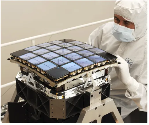
図
1.9:
衛 星 搭 載 前 の1.4m
ミ ラ ー 。ク リ ー ン ル ー ム に て 。http://www.ballaerospace.com/gallery/kepler/gallery5.htm
1.2.4
焦点面アレイ測光器の心臓部を為すのが焦点面アレイであり、
CCD、サファイア製の焦点面平滑化レンズ、
インバー基盤、ヒートパイプ、ラジエータで構成されている。各

![図 3.3: MCMC で得られた公転周期 P の分布。横軸は公転周期 P [日]、縦軸は頻度。](https://thumb-ap.123doks.com/thumbv2/123deta/10115228.1949217/30.892.196.694.811.1132/図33MCMCで得られた公転周期Pの分布横軸は公転周期P日縦軸頻度.webp)
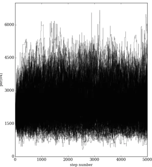
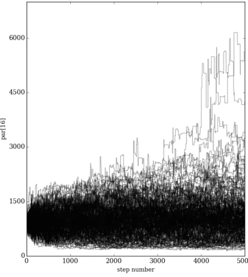
![図 3.6: MCMC における公転周期 P の chain に対する進化。横軸は chain、縦軸は公転周期 P [日]。](https://thumb-ap.123doks.com/thumbv2/123deta/10115228.1949217/33.892.198.693.177.711/図36MCMCにおける公転周期Pのに対する進化横軸縦軸公転周期日.webp)


![図 3.27: MCMC で得られた公転周期 P の分布。横軸は公転周期 P [日]、縦軸は頻度。](https://thumb-ap.123doks.com/thumbv2/123deta/10115228.1949217/51.892.193.699.817.1137/図327MCMCで得られた公転周期Pの分布横軸は公転周期日縦軸頻度.webp)