Visual Docking of Underwater Vehicle

(1)

Visual Docking of Underwater Vehicle

Under Turbid and Day/Night Lighting Environment

岡山大学大学院自然科学研究科博士後期課程産業創成工学専攻

（平成 3 0 年度）

学生番号 51427357 Khin Nwe Lwin

(2)

Under Turbid and Day/Night Lighting Environment

Intelligent Robotics and Control Laboratory Khin Nwe Lwin (51427357)

Abstract ：

Autonomous underwater vehicles (AUVs) play an important role in human society in diﬀerent applications such as inspection of underwater structures (dams, bridges), ship hull inspections, and scientiﬁc studies of the deep ocean. However, underwater vehicle operations are limited to activities that can be completed in short duration time, which is caused by the limited power capacity of batteries set on the vehicles. Even though advanced technology related to power devices provides long operation periods, underwater vehicles must come back to a surface vessel for recharging when operations take more than a couple of days. A recharging function that needs the AUVs to be docked to the recharging station can enable the AUVs to operate in extended period in an actual sea without returning surface vehicle for recharging. Therefore, underwater recharging system with a docking function have been researched using various approaches.

Most researches have used single camera for docking. On the other hand, the precision of distance measurement in the camera depth direction is not enough to accomplish the docking by AUVs in which high homing accuracy is indispensable. To overcome this problem, the author has proposed a new 3D-perception-based move-on-sensing (3D-MoS) system with stereo vision cameras for underwater battery recharging. The visual servoing of an underwater vehicle using the parallactic nature of stereoscopic vision and 3D-model- based recognition and real-time multi-step genetic algorithm (RM-GA) was initiated by our research group.

This thesis proposes the improvement of the dynamic performance of real-time 3D pose tracking by tuning RM-GA parameters and conﬁrming optimization of the dynamic

(3)

of RM-GA have been selected based on some analyses on their performance to improve the proposed system especially in terms of convergence time and recognition accuracy.

After optimizing the RM-GA parameters, the performance of the proposed system was conﬁrmed, enhancing the tolerance against the turbidity in the actual sea environment.

The experimental results conﬁrmed that the proposed RM-GA system with the optimum parameters can improve the real-time recognition performance and closed-loop dynamics of visual feedback control.

Additionally, the turbidity tolerance of the proposed system using the current non- lighting 3D marker has been limited to some level of turbidity and lighting changing environments. According to the authors’ knowledge, no existing study has conducted the docking using stereo-vision-based real-time visual servoing with performance tolerance of turbidity and illumination varieties. Since underwater battery recharging units are installed in the deep-sea bottom, the deep-sea docking cannot avoid the influence of the turbidity and low light environment. When the current non-lighting 3D marker is lighted by vehicle’s LED in turbid water environment, the images taken by two cameras set on the vehicle look wholly white, some new idea seems to be required. The lighting from the vehicle has been confirmed not to be effective method to detect something in turbid and dark condition. To overcome the above situation, a newly designed lighting marker (active 3D marker) that has LEDs inside was devised in this study.

Based on the above motivation, the experiments have been conducted to verify the robustness of the proposed docking approach in the simulated pool where the turbidity of the water and the lighting were varied. Then, the eﬀectiveness of the proposed stereo vision control system has been evaluated from the viewpoints of practicality and functionality in natural environments by conducting the docking experiments in the presence of turbidity in the actual sea. We have conﬁrmed:

(1) The eﬀectiveness and practicality of the real-time 3D pose estimation system by conducting a sea docking experiment using the optimum RM-GA parameters.

(4)

marker in the actual sea with dark and turbid environment.

The experimental results confirmed that the proposed system can provide high homing accuracy in dark and turbid environment. The successful docking operations using stereo vision cameras and 3D lighting marker have confirmed the proposed system to be effective for realizing a long duration time for autonomous intelligent robots to collect automatically rare metals at the bottom of the deep-sea.

(5)

List of Figures

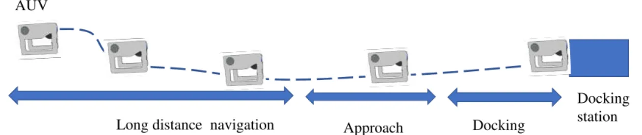
2.1 Underwater AUV docks into the docking station. The docking process generally involves (1) long distance navigation, (2)approaching, and (3) docking. . . 15 2.2 Diﬀerent AUVs used for docking experiments: (a) Starbug AUV [6], (b)

Girona 500 AUV [4], and (c) Tuna-Sand 2 AUV [103]. . . 15 2.3 Diﬀerent homing methods: (a) homing using docking net mechanism, (b)

homing using a manipulator, and (c) proposed homing method with docking pole and docking hole. . . 18 2.4 Diﬀerent docking structures : (a) Omnidirectional docking, (b) Unidirec-

tional docking. . . 19 2.5 Diﬀerent optical systems : (a) Using light sources [26], (b) Using structured

patterns [6]. . . 21 2.6 (a) Correct an incorrect mapping in 2D-to-3D space and (b) pairing of

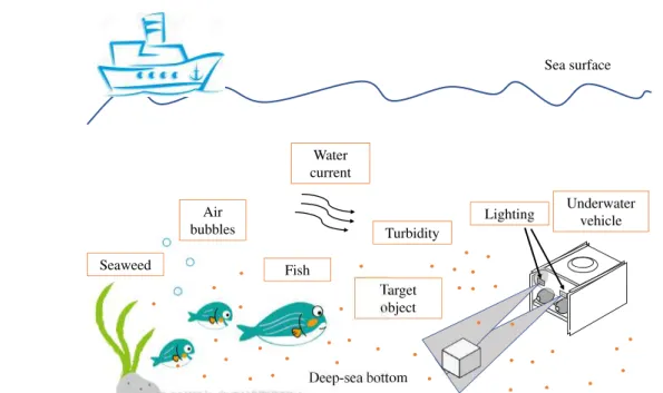
points in 3D-to-2D projection. . . 24 2.7 Evolution process in GA. . . 29 2.8 Visual servoing in a deep-sea environment with disturbances such as current

wave, turbidity, illumination (natural light and vehicle’s light), and obstacle (such as ﬁsh, seaweed, air bubbles). . . 31 3.1 A 3D-MoS based robotic system in which the free space is estimated for

every movement by sensing the relative pose using stereo vision. . . 36

(10)

cepts of 3D-to-2D projection and 2D-to-3D reconstruction. . . 38 3.3 A 3D marker consists of three spheres 40 mm in diameter and colored red,

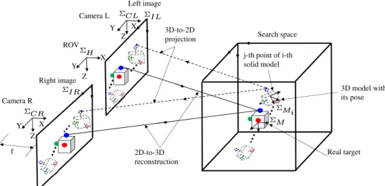
green, and blue. . . 38 3.4 Perspective projection of dual-eyes vision-system: In the searching area,

a 3D solid model is represented by dotted point (jth photo-model). The coordinate systems of photo-model, camera and image are represented by Σ_M_j, Σ_CL, Σ_CR, Σ_IL and Σ_IR respectively. A 3D solid model that is assumed to be in the searching area is projected from 3D space to 2D left and right camera images. . . 39 3.5 Projection Matrix. . . 44 3.6 Real 3D marker and i-th 3D model projected to left camera’s 2D space. . . 47 3.7 Fitness distribution. The peak represents the true pose detected by the

designed fitness function. The noise, which represents incorrect poses, is generated in the fitness distribution as a result of image deformation caused by environmental effects. . . 49 3.8 Structure of RM-GA chromosome: 12 bits each for x, y, and z represent

the position coordinates of the 3D model, and 12 bits each for²₁, ²₂, and ²₃ describe the orientation deﬁned by a quaternion. The resolution for x and y are 0.20 mm, z is 0.10 mm, and ²₃ is 0.013^◦. . . 52 3.9 (a) ﬂowchart of process steps while the genes converge to the target 3D

marker from the ﬁrst to the ﬁnal generation and (b) graphical representa- tion of solution evaluation and chromosome evolution during each 33-ms control period. The RM-GA converges to the solution in successively input dynamic images. . . 53 3.10 Underwater target and GA searching space. . . 54 3.11 Overview of ROV (a) front view (b) side view (c) top view (d) back view. . 56

(11)

hole. . . 56 3.13 Block diagram of visual servo control. °A in this ﬁgure represents output

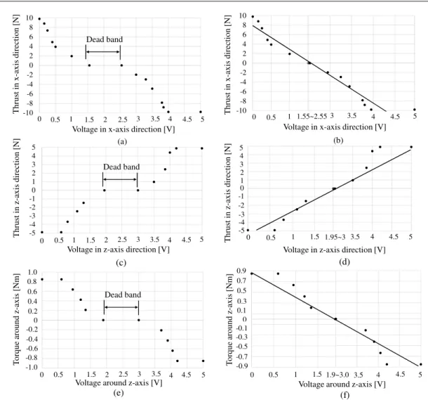
of pose estimated by RM-GA, which corresponds to °C Fig. 3.9. . . 59 3.14 Left column shows initial characteristics of thrust or torque against con-

trol voltage and the right column shows adjusted characteristics by removing the dead band and linearization: (a) initial characteristics in x-axis direction, (b) characteristics after removing dead band (black dots) and adjusting (solid line) in x-axis direction, (c)(d) initial and adjusted characteristics in z-axis direction, and (e)(f) initial and adjusted characteristics around z-axis. . . 60 3.15 Passive marker and active marker. In passive marker, lighting is emitted

from the ROV. In active marker, lighting is emitted from the 3D marker that has LEDs inside of each sphere. . . 62 3.16 Active/Lighting 3D marker and its internal circuit diagram: red, green and

blue LEDs were installed inside the white spherical ball, and each ball is covered by each color balloon. The resistance value of the variable resistors, and the number of resistors are determined by trial and error. . . 62 4.1 Layout of experiment using 3D marker and two cameras. . . 64 4.2 Number of generations created by RM-GA within 33 ms based on diﬀerent

chromosome population sizes. . . 65 4.3 Comparison of convergence time for ﬁtness value of 0.6 and population size

of 10 with diﬀerent selection and mutation rates: selection rates = 0.2, 0.4, 0.6, and 0.8 and mutation rates = 0.05, 0.1, and 0.15. The vertical dotted line “A” shows the convergence time of the best combination of RM-GA parameters for a population of 10. The parameters of “A” are given in Table 7.1. . . 66

(12)

of 20 with diﬀerent selection and mutation rates: selection rates = 0.2, 0.4, 0.6, and 0.8 and mutation rates = 0.05, 0.1, and 0.15. The vertical dotted line “B” shows the convergence time of the best combination of RM-GA parameters for a population of 20. The parameters of “B” are given in Table 7.1. . . 67 4.5 Comparison of convergence time for ﬁtness value of 0.6 and population size

of 40 with diﬀerent selection and mutation rates: selection rates = 0.2, 0.4, 0.6, and 0.8 and mutation rates = 0.05, 0.1, and 0.15. The vertical dotted line “C” shows the convergence time of the best combination of RM-GA parameters for a population of 40. The parameters of “C” are given in Table 7.1. . . 68 4.6 Comparison of convergence time for ﬁtness value of 0.6 and population size

of 60 with diﬀerent selection and mutation rates: selection rates = 0.2, 0.4, 0.6, and 0.8 and mutation rates = 0.05, 0.1, and 0.15. The vertical dotted line “D” shows the convergence time of the best combination of RM-GA parameters for a population of 60. The parameters of “D” are given in Table 7.1. . . 69 4.7 Comparison of convergence time for ﬁtness value of 0.6 and population size

of 80 with different selection and mutation rates: selection rates = 0.2, 0.4, 0.6, and 0.8 and mutation rates = 0.05, 0.1, and 0.15. The vertical dotted line “E” shows the convergence time of the best combination of RM-GA parameters for population 80. The parameters of “E” are given in Table 7.1. 70 4.8 Comparison of effect of optimal primary parameters on fitness value for

population sizes of 10, 20, 40, 60, and 80 and increased calculation time.

Values for selection and mutation rates are given in Table 7.1. . . 71 4.9 Layout of the station for sea docking. . . 72

(13)

sults for the times corresponding to lines “A”-“F” are given in Fig. 5.17. . 75 4.11 Docking experiment in actual sea environment with turbidity: (a) position

in x-axis direction, (b) position in y-axis direction, (c) position in z-axis direction, and (d) orientation around z-axis. The dotted lines “A”-“F”

in each panel correspond to docking stages as follows: (A) end of manual operation, (B) transition to visual servoing, (C) start of docking, and (D-F) completion of docking. Photographs taken at these times are shown in Fig.

5.18. . . 76 4.12 Photographs of docking experiment in actual sea environment with turbid-

ity and position in x-axis direction: Each panel corresponds to the time denoted dotted lines “A”-“F” in Fig. 5.17. Note the placement of the docking pole in the docking hole in photograph ”F.” In each panel, the upper photographs are the left and right camera images acquired by the ROV and the lower photographs were taken by two underwater monitoring cameras (back view and top view of docking hole from cameras inside the docking station). . . 77 4.13 All genetic data analyses: (a) position of all genes for x-axis, (b) position

of all genes for y-axis, (c) position of all genes for z-axis, and (d) position of all genes for orientation around z-axis. . . 78 4.14 Top genes (60 %) data analyses: (a) position of top genes for x-axis, (b)

position of top genes for y-axis, (c) position of top genes for z-axis, and (d) position of top genes for orientation around z-axis. The top genes are ranked and selected to represent the true pose. . . 79 4.15 Bottom genes (40 %) data analyses: (a) position of bottom genes for x-axis,

(b) position of bottom genes for y-axis, (c) position of bottom genes for z-axis, and (d) position of bottom genes for orientation around z-axis. . . . 79

(14)

for y-axis, (c) mean value for z-axis, and (d) mean value for orientation around z-axis. The shape of the mean value is similar to the shape of top gene’s pose in Fig. 4.14. . . 80 4.17 Standard deviation of all genes analyses: (a) standard deviation for x-axis,

(b) standard deviation for y-axis, (c) standard deviation for z-axis, and (d) standard deviation for orientation around z-axis. . . 80

5.1 Distribution of the top 36 genes in the case of a plain background: (a) position in the x direction, (b) position in the y direction, (c) position in the z direction, (d) orientation around the z-axis, (e) left and right camera images at 10 s from the beginning of the experiment, and (f) left and right camera images at 40 s from the beginning of the experiment in the presence of air bubble disturbance. . . 85 5.2 Distribution of the top 36 genes in case of a simulated ocean background:

(a) position in the x direction, (b) position in the y direction, (c) position in the z direction, (d) orientation around the z-axis, (e) left and right camera images at 10 s after the beginning of the experiment, and (f) left and right camera images at 40 s after the beginning of the experiment in the presence of air bubble disturbance. . . 86 5.3 Fitness distributions generated by scanning the assumed pose value in y-z

plane and x-y plane with plain background at 10 s and 40 s after the start of the experiment in the presence of air bubble disturbance: (a) fitness distribution between the y and z positions at 10 s, (b) fitness distribution between the y and z positions at 40 s, (c) fitness distribution between the y and x positions at 10 s, and (d) fitness distribution between the y and x positions at 40 s. . . 89

(15)

plane and x-y plane with simulated ocean background sheet at 10 s and 40 s after the beginning of the experiment in the presence of air bubbles:

(a) fitness distribution between the y and z positions at 10 s, (b) fitness distribution between the y and z positions at 40 s, (c) fitness distribution between the y and x positions at 10 s, and (d) fitness distribution between the y and x positions at 40 s. . . 90 5.5 Regulation performance of visual servoing by dual-eye image recognition

with plain background without air bubble disturbance: (a) ﬁtness value, (b) error in the x direction, (c) error in the y direction, (d) error in the z direction, (e) error around the z axis, (f) 3D trajectory of underwater vehicle, (g) thrust in the x direction, (h) thrust in the y direction, (i) thrust in the z direction, and (j) thrust around the z-axis. . . 93 5.6 Regulation performance of visual servoing by dual-eye image recognition

with plain background with air bubble disturbance: (a) ﬁtness value, (b) error in the x direction, (c) error in the y direction, (d) error in the z direction, (e) error about the z-axis, (f) 3D trajectory of the underwater vehicle, (g) thrust in the x direction, (h) thrust in the y direction, (i) thrust in the z direction, and (j) torque about the z-axis. . . 94 5.7 Setup of visual servoing experiment with periodic motion of 3D marker. . 95 5.8 Tracking performance of dual-eye image recognition with plain background

without air bubble disturbance for the case in which “(A)” the 3D marker moves in the x direction with an amplitude of 280 mm and a period of 20 s after 20 s have passed from the start: (a) ﬁtness value, (b) position of the underwater vehicle in the x direction (dashed line is the desired position), (c) tracking error in the x direction, and (d) thrust in the x direction.

Photographs were taken every 10 s during this experiment and are shown in Fig. 5.11. . . 96

(16)

without air bubble disturbance for the case in which “(A)” the 3D marker moves in the x direction with an amplitude of 280 mm and a period of 15 s after 20 s have passed from the start: (a) ﬁtness value, (b) position of the underwater vehicle in the x direction (dashed line is the desired position), (c) tracking error in the x direction, and (d) thrust in the x direction. . . . 97 5.10 Tracking performance of dual-eye image recognition with plain background

without air bubble disturbance for the case in which “(A)” the 3D marker moves in the x direction with an amplitude of 280 mm and a period of 10 s after 20 s have passed from the start: (a) ﬁtness value, (b) position of the underwater vehicle in the x direction (dashed line is the desired position), (c) tracking error in the x direction, and (d) thrust in the x direction. . . . 98 5.11 Photographs of the underwater vehicle (left column) and captured images

from the ROV (right column) without disturbances. These photographs correspond to the results shown in Fig. 5.8: (a) 10 s have passed (without making the 3D marker move after starting experiment), (b) 20 s have passed (backward moving 3D marker), (c) 30 s have passed (forward moving 3D marker), (d) 40 s have passed (backward moving 3D marker), and (e) 50 s have passed (forward moving 3D marker). . . 100 5.12 Tracking performance of dual-eye image recognition with plain background

with air bubble disturbance for the case in which “(A)” the 3D marker moves in the x direction with an amplitude of 280 mm and a period of 20 s after 20 s have passed from the start and “(B)” disturbances are generated after 10 s: (a) ﬁtness value, (b) position of the underwater vehicle in the x direction (dashed line is the desired position), (c) tracking error in the x direction, and (d) thrust in the x direction. Photographs were taken every 10 [s] during this experiment and are shown in Fig. 5.15. . . 101

(17)

with air bubble disturbance for the case in which “(A)” the 3D marker moves in the x direction with an amplitude of 280 mm and a period of 15 s after 20 s has passed from the start and “(B)” disturbances are generated after 10 s: (a) ﬁtness value, (b) position of the underwater vehicle in the x direction (dashed line is the desired position), (c) tracking error in the x direction, and (d) thrust in the x direction. . . 101 5.14 Tracking performance of dual-eye image recognition with plain background

with air bubble disturbance for the case in which “(A)” the 3D marker moves in the x direction with an amplitude of 280 mm and a period of 10 s after 20 s has passed from the start and “(B)” disturbances are generated after 10 s: (a) ﬁtness value, (b) position of the underwater vehicle in the x direction (dashed line is the desired position), (c) tracking error in the x direction, and (d) thrust in the x direction. . . 102 5.15 Photographs of the underwater vehicle (left column) and captured images

from the ROV (right column) with disturbances. These photographs correspond to the results shown in Fig. 5.12: (a) 10 s have passed (without making the 3D marker move or air bubble disturbances after starting the experiment), (b) 20 s have passed (backward moving 3D marker), (c) 30 s have passed (forward moving 3D marker), (d) 40 s have passed (backward moving 3D marker), and (e) 50 s have passed (forward moving 3D marker). 103 5.16 Visual servoing experiment with bubble disturbances between the ROV

and the 3D marker, and layout of the docking experiment. The ROV is with a rod (8 mm × 6 mm) on its right-hand side, and the 3D marker is with a docking hole having a radius of 35 mm on its left-hand side. The center distance between the docking hole and the 3D marker was 145 mm.

Two instruments were designed to intermittently generate bubbles in the water using air pumps. . . 104

(18)

image recognition: (a) ﬁtness value, (b) position along the x-axis, (c) position along the y-axis, (d) position along the z-axis, (e) orientation around the z-axis, (f) detected 3D pose of the underwater vehicle by RM-GA, (g) voltage along the x-axis, (h) voltage along the y-axis, (i) voltage along the z-axis, and (j) voltage around the z-axis. The dotted lines denoted by

“A,” “B,” and “C” in each of the subﬁgures indicate the start of visual servoing, the start of docking, and the completion of docking, respectively.

Photographs taken at these times are shown in Fig. 5.18. . . 106

5.18 Photographs of docking (left column) and dual-eye camera images from the ROV (right column) with air bubble disturbance: (a)-(b) 0 s - 4 s visual servoing state, (c)-(e) 8 s - 16 s docking process, and (f)-(h) 20 s- 25 s completion of docking. Each ﬁgure corresponds to the experimental results shown in Fig. 5.17, where the corresponding times are indicated by dotted lines “A,” “B,” and “C,” respectively. . . 108

5.19 Experimental setup of sea docking. The two underwater cameras, (1) back camera and (2) top camera, were attached to the docking station to monitor the behavior of the ROV. . . 111

5.20 Layout of the sea docking experiment. (a) ROV is controlled by the RM-GA PC while its behavior is monitored by the recording PC. (b) Left camera image of the ROV showing the 3D marker and docking hole located in the docking station. The center distance between the docking hole and 3D marker was 145 mm. (c) Position of ROV and docking station, which was a rectangular cuboid with length of 600 mm, width of 450 mm, and height of 3,000 mm. The photograph (c) represents the completion of docking. . . 112

(19)

position in the x-axis direction during 4 docking iterations in the sea. The upper photos represent the left and right cameras images set at the ROV taken at visual servoing stage, docking stage and completion of docking stage. The lower photos are images taken by the underwater cameras set at the docking station at the same stages of docking process. Detailed results for the docking experiment°1 is presented in Fig. 5.22and the photographs of the docking experiment°1 is shown in Fig. 5.23. The dotted line shows the returning procedure from docking completion position to restarting position of visual servoing, the ROV’s returning motion took about 6 s. . . 113 5.22 Docking performance in a actual sea for the ﬁrst time docking indicated by

°1 of Fig. 5.21: (a) ﬁtness value, (b) position along the x-axis, (c) position along the y-axis, (d) position along the z-axis, (e) orientation around the z- axis, (f) detected 3D pose of the underwater vehicle by RM-GA, (g) voltage along the x-axis, (h) voltage along the y-axis, (i) voltage along the z-axis, and (j) voltage around the z-axis. The dotted lines denoted by “A”-“H”

in each of the subﬁgures indicate the time during the ﬁrst time docking of Fig. 5.21. Photographs taken at these times are shown in Fig. 5.23. . . 114 5.23 First column shows the photographs of docking monitor by station back

camera. Second column represents the photographs of docking monitor by station top camera. Third and fourth columns describe the ROV’s left and right cameras images: “A”-“C” (0 s - 3 s) visual servoing state, “C”-“H”

(8 s - 50 s) docking operation. Each ﬁgure corresponds to the experimental results shown in Fig. 5.22, where the corresponding times are indicated by dotted lines “A”-“H,” respectively. Especially, it can be conﬁrmed from image that the end of docking pole was inserted in docking hole at time “H”.116 6.1 Docking station with a 3D marker and a docking hole . . . 120

(20)

6.3 Layout of docking experiment and description of the alignment process between the ROV and 3D marker: (a) Desired pose in visual servoing state and (b) Desired pose in docking completion state. . . 123 6.4 Appearance of the testing pool. . . 123 6.5 Pool docking results: (a) Fitness value; (b) Photograph of ROV after dock-

ing completion; (c), (e), (g), (i) Recognized positions along the x-, y-, and z-axis directions and rotation around the z-axis, respectively; where the desired values for visual servoing state are given as x_d = 600 mm, y_d = 0 mm, z_d = -30 mm, ε_3d = 0^◦; and (d), (f), (h), (j) Voltage commanding thrust in the x-, y-, and z-axis directions and rotation around the z-axis, respectively. . . 127 6.6 Sea docking results: (a) Fitness value; (b) Photograph of ROV in docking

completion; (c), (e), (g), (i) Recognized positions along the x-, y-, and z-axis directions and rotation around the z-axis, respectively; where the desired values for visual servoing state are given as xd = 600 mm,yd = 12 mm,z_d= -70 mm, ε_3d = 0^◦ ; and (d), (f), (h), (j) Voltage along the x-, y-, and z-axis directions and rotation around the z-axis, respectively. “A” and

“B” correspond to Fig. 6.7(d), (e), indicated as “C.” . . . 128 6.7 Periodically captured images from dual-eye cameras during the docking op-

eration and corresponding images from underwater camera installed in the docking station: (a),(b) Images of manual control, (c)-(e) Images of visual servoing, and (f)-(i) Images of docking. Dotted circles in dual-eye camera images are the poses recognized by RM-GA. The images labeled with (C) correspond to the results shown in Fig. 6.6(e), (i) that are indicated by

“A” and “B,” respectively. . . 129 7.1 Dual eyes vision-based docking system in Tuna-Sand 2 . . . 132

(21)

7.3 Docking station structure which includes a 3D maker, a docking hole, underwater cameras to observe experimental conditions. . . 135

7.4 (a) Layout of docking experiment, (b) Coordinate system of Tuna-Sand 2 . 136

7.5 Flowchart of GA-PC command behavior in which TS2 means Tuna-Sand2. 137

7.6 Layout of the AUV and docking station in which the actual position and target position are illustrated to explain how to calculate the command value to be sent to Tuna-Sand2. . . 138

7.7 Flowchart of three steps in docking experiment: error in z-axis is compensated in Mode 51. Then, errors in x-y plane are compensated in Mode 52.

Finally angular error around z-axis is compensated in Mode 53. . . 140

7.8 Detailed ﬂowchart of GA-PC. . . 148

7.9 Subﬂowchart of Visual Servoing in Fig.7.8 . . . 149

7.10 Appearance of experimental environment to conduct automatic docking using AUV Tuna-Sand 2 in water pool established in University of Tokyo. . 150

7.11 Layout of 3 times docking pretests using only visual servoing. The number in circle °1 - °3 represents for docking iteration. After each docking completion, the AUV moves to the posse as shown in this ﬁgure for next docking. Experimental results are shown in Fig.7.12and corresponding left and right camera images are illustrated in Fig. 7.13. . . 150

(22)

position along in x-direction, (c) position along y-axis direction, (d) position along z-axis direction, and (e) rotation around z-axis. The number in each circle in each subﬁgure represents docking number. Note the AUV moves to the poses as shown in Fig. 7.11after each docking completion.

The initial poses for docking number °2 and docking number °3 are set by giving oﬀset especially in y-axis direction after moving back process as shown by times A1 and A2 (see Fig.7.12(c): The 3D marker is in the negative position of y-axis direction of Σ_H for the docking number °² as shown in Fig. 7.11, and the 3D marker is in the positive position of y-axis direction of ΣH for the docking number°³ as shown in Fig. 7.11). Left and right camera images taken at the times “A”-“H” are shown in Fig. 7.13. . 151 7.13 Left and right camera images corresponding to the times A-H in Fig. 7.12.

It can be conﬁrmed that the AUV could perform docking by visual servoing in pretests by checking the left and right images taken at the times “A”-

“H”. Subﬁgures 7.13(“A,” “D,” “G”) show the condition in which the AUV is stable and ready of docking. Subﬁgures 7.13(“B,” “E,” “H”) show the condition in which docking is completed. . . 152 7.14 Desired trajectory of Tuna-Sand 2 in experiment and appearance of Tuna-

Sand2: From (a) to (i), appearance of experiments are shown during movement of trajectory which is illustrated in (j). Terminal positions of those trajectory are described in Table 2. . . 153 7.15 Measured trajectory of Tuna-Sand2 by GA-PC with RM-GA: Fitness value

is plotted in (a). When ﬁtness value is low, reliability for measured position is lower. AUV positions in x,y and z axes are plotted in (c), (d) and (e) respectively. Also, rotation angle around z axis is plotted in (f). When those control variables were converged in acceptable range on visual servo state at about 83 second, docking behavior is executed. . . 154

(23)

per graph indicates ﬁtness value with respect to time during docking scheme.

(i), (ii) and (iii) in this graph mean instants which are picked up for draw- ing ﬁgures in lower side. Pose relations between AUV and 3D maker in those instants (i, ii, iii) are illustrated in second row. Distribution map with Y-X axes and a pose estimated by proposed GA algorithms are drawn in third row, and that with Y-Z axes and estimated pose are also drawn in ﬁnal row. . . 155

7.17 Quotanion (a) ²1 around x_H , (b) ²2 around y_H , (c) ²3 around z_H are illustrated. It can be conﬁrmed that rotation angle around x_H and y_H are stable that are out of control targets. . . 156

8.1 The experimental set-up in the case of night-time condition: (a) ROV and an active marker in the simulated pool, (b) left and right cameras images from which the dotted circles represent the real-time estimated pose by the proposed system. . . 160

8.2 Flowchart of the docking strategy. In pool test, the manual approach and the stay step were not performed. After completion of docking step, the ROV stops visual servoing and stores the data ﬁles from memory into the hard disk. . . 161

8.3 Fitness values against turbidity at the distance 600 mm between the ROV and 3D marker. The illumination for day and night time are 1280 (lx) and 80 (lx) respectively. The left and right camera images taken at (A), (B), (C) are shown in Fig. 8.4. . . 164

(24)

Fig.8.3for day and night time. Dotted cycles mean recognized poses by RM-GA. Even though the currents of red, blue, green LEDs are ﬂowing in day and night conditions, they look not lighting in daytime and look lighting in night-time. . . 165

8.5 (a) Layout of the pool docking experiment. (b) Pool docking coordinate system. . . 166

8.6 Illumination simulated for each docking time. Lighting condition is changed from daytime to night-time gradually. . . 167

8.7 Docking performance against turbidity 10 (FTU) under 1280 (lx) (maximum lighting condition): (a) ﬁtness value, (b) position along the x-axis, (c) position along the y-axis, (d) 3D trajectory of the underwater vehicle, (e) position along the z-axis, and (f) orientation along the z-axis. . . 168

8.8 Docking performance against turbidity 10 (FTU) under 80 (lx) (minimum lighting condition): (a) ﬁtness value, (b) position along the x-axis, (c) position along the y-axis, (d) 3D trajectory of the underwater vehicle, (e) position along the z-axis, and (f) orientation along the z-axis. . . 169

8.9 Layout of the station for sea docking. The ROV is controlled by GA-PC and the behavior of the ROV is monitored by recording PC. . . 171

8.10 Layout of sea docking coordinate system. The two underwater cameras are attached inside the docking station for monitoring the behavior of the ROV. 172

8.11 Enlarge view of Fig. 15 (b) and (c) to see clearly the desire position in the x-axis. . . 172

(25)

(a) ﬁtness value, (b) position along the x-axis, (c) position along the y-axis, (d) position along the z-axis, (e) orientation around the z-axis, (f) 3D trajectory of the underwater vehicle, (g) voltage along the x-axis, (h) voltage along the y-axis, (i) voltage along the z-axis, (j) voltage around the z-axis, (k) corresponding photographs taken at the time “A”, (l) corresponding photographs taken at the time “E”, and (m) corresponding photographs taken at the time “G”. The dotted lines “A”-“G” in each subﬁgure correspond to docking stages as follows: (A-C) transition to visual servoing, (D) start docking, (D-G) completion of docking. The lower photographs (k), (l), (m) were taken at the same time by left and right cameras of ROV (1), (2) and two underwater monitoring cameras (3), (4) (top view and side view of docking hole). The positions of the two underwater cameras (3)-(4) are shown in Fig. 8.10. . . 174

(26)

(27)

List of Tables

3.1 Parameters of the Real-time Multi-step GA . . . 55 3.2 Speciﬁcation of ROV . . . 57 4.1 Primary parameter values that produced the fastest convergence time for

each population size with a ﬁtness value of 0.6. . . 69 4.2 Optimum parameters for RM-GA. . . 70 5.1 Position recognition accuracy of top genes in the presence or absence of air

bubble disturbances for the case of with and without background sheet. . . 88 7.1 Speciﬁcation of Tuna-Sand 2 . . . 134 7.2 Points for desired trajectry of Tuna-Sand2 in Fig.7.14. Coordinate system

of these position is ΣW that is drawn in Fig.7.14(j) . . . 142

(28)

Chapter 1 Introduction

Japan has huge sea area from which resources can be taken out using advanced tech- nologies. Autonomous underwater vehicle (AUV) plays an important role in deep-sea works such as oil pipe inspection, survey of seafloor, searching rare metal, etc [1]-[5]. The Japanese government is now seriously considering searching methane hydrate as a future energy solution. To do such novel works that need long duration time in the deep sea, one of the main limitations of AUVs is limited power capacity. Since the electricity of AUVs is supplied by the battery for AUV’s moving around the sea floor, AUVs have to float to the sea surface for recharging if the power capacity of AUV is not enough for tasks that take longer operation. Therefore, decreasing the working time and dropping the work efficiency in the deep-sea became the problems for deep-sea applications where operations take a couple of days. To solve these problems, underwater battery recharging technology with docking function is one of the solutions even though challenges are still remained.

In a docking-based battery recharging system, the power supply facility is installed in the seabed in which the AUV automatically charges without going to the sea surface and it can do tasks continuously for a long time. Moreover, docking function takes place as an important role not only for battery recharging but also for other advanced applications such as intervention using some manipulators. Therefore, the important task of docking work is to connect the charging facility and the AUV.

(29)

This thesis presents a new method to deal with the docking for AUVs. In the ﬁrst part of this thesis, the performance of the proposed system using stereo vision for real-time pose tracking was discussed and improved by tuning the real-time multi-step GA (RM-GA) parameters. In the second part of this thesis, the stability of the closed-loop dynamics of an ROV with real-time pose feedback when the deformation on the cameras images imposed by air bubbles was explored by analyzing the RM-GA’s behavior. In the third part of this thesis, the docking experiments using the proposed approach that simulate for underwater battery recharging were conducted in the sea, near Wakayama City, Japan.

The sea docking was conducted using an ROV as a test bed successfully. To confirm the effectiveness of the proposed docking system with a fully autonomous AUV, the docking experiment using hovering type AUV (Tuna-Sand 2: University of Tokyo) is presented in the fourth part of this thesis. The experimental results proved that the proposed system using the current non-lighting 3D marker is effective and feasible for underwater battery recharging. However, when the ROV operates in turbid water environment and night condition, the lighting from the vehicle has been confirmed not to be effective method.

Therefore, a newly active/lighting 3D marker was devised to overcome the above situation of the proposed system. On the other hand, point light marker with no lighting from the ROV has been sometimes used for pose estimation, which is possibly hidden by small sea weeds or something easily. Point light marker is only a point and there is no changing the size of view when the vehicle was neared or far away from the docking station. The solid 3D marker has the color, shape, and diameter information. Therefore, when the vehicle neared the docking station, the size of the 3D marker is bigger and bigger. It has the changing size of view depended on the distance form the vehicle. The proposed system that composes the optimum RM-GA parameters and the new active/lighting 3D marker under turbidity and illumination variation for real-time pose estimation was explained in the ﬁnal part of this thesis. The experimental results conﬁrmed that the proposed system can provide high homing accuracy and robustness against turbidity that enables the vehicle dock to a recharging station set at sea bottom. The successful docking operations using

(30)

stereo vision cameras and 3D lighting marker have conﬁrmed the proposed system to be eﬀective for realizing a long duration time for autonomous intelligent robots to collect automatically rare metals at the bottom of the deep-sea.

1.1 Background and Motivation

A number of studies have examined control and guidance systems for underwater vehicles [6]-[9]. Robust vision-based target identification and homing using self-similar landmarks (SSLs), which enables robust target pose estimation using a single camera, has been proposed [6]. The pose of an AUV measured using an electromagnetic homing system has also been investigated [7]. In [4], Girona 500 AUV was developed for inspection and intervention tasks for the seafloor survey. In that work, several sensors such as sonar, GPS, pressure sensor, velocity, fiber optic gyro, and plural video cameras are used to localize an object. But the cameras look at different targets, so these approaches do not realize parallactic nature. In the approach of [8], an autonomous docking system for intervention using sonar and video camera system was developed. After performing the docking operation, the manipulator turns valves. The autonomous underwater manipulator for intervention mission in the oceanic environment was developed by SAUVIM [9]. Recently, vision-based systems for underwater vehicles have been studied for different applications [10]-[25]. Even though the vision-based approach is restricted to short-range measurement, and it degrades in the presence of turbidity and bubbles made by waves, it has the potential for the detection of three-dimensional (3D) poses that is essentially necessary for docking a vehicle precisely.

Most studies on guidance techniques using cameras for homing or docking operations are based on monocular vision to acquire the distance between a target and a vehicle [10], [11]. The reliable pose estimation of underwater docking using a single camera through a scene invariant approach was proposed in [12]. The methodology in [12], however, is thought to be diﬃcult for real-time pose estimation, and it has not been applied to

(31)

docking. An autonomous underwater torpedo-type vehicle was optically guided by lights mounted around the entrance of a docking station using one camera in [13]. A docking method for hovering type AUVs using one camera based on both acoustic and visual positioning was proposed in [14]. The merit of the monocular camera is that the conﬁgu- ration is simple, and processing time seems to be less than that of the multi-cameras unit.

The disadvantage is that the precision of distance measurement of the camera’s depth direction is not enough for applications in which high homing accuracy is required.

To overcome the limitation of single-camera-based systems, there are some studies using two cameras [15]-[20]. Binocular vision was used in some of these studies in order to detect the position of the vehicle and dock with a station [15]-[18]. In [15], AUV docks autonomously into a funnel-shaped docking station and then a vehicle-mounted manipulator performs several given tasks. In spite that two cameras have been mounted on the vehicle, one looking forward to estimate panel pose and the other pointing down to help the mounted manipulator conduct some tasks. In [16], even though two cameras were used, one was facing downward and the other was looking forward for the purpose of obstacle avoidance and docking. A vision system for autonomous guidance using two cameras to track separate artiﬁcial underwater landmarks was proposed in [17]. In another study, the vehicle position was estimated using two cameras and a sonar system [18]. In that approach, the position of the vehicle was calculated by combining data from Doppler sonar and CCD cameras, which does not deal with the orientation for controlling the vehicle. In two of the studies mentioned above [15], [16], “stereo vision” was not used even though two cameras were used. On the other hand, a concept of “stereo-vision” that authors conceive implies a method to have a 3D space perception by having plural images of one target object, which enables the pose estimation to exploit parallactic nature.

To extend the persistence time of an underwater operation, the authors have proposed a new 3D pose estimation method with dual-eye vision-based docking approach that exploits the parallactic nature of stereoscopic vision to enable reliable 3D pose estimation in real time by avoiding the limitations of the above mentioned studies. A pose estimation

(32)

approach based on 3D-to-2D model projection was applied in this study because the forward projection from 3D-to-2D generates unique points in 2D images without any errors meaning that the issue of incorrect mapping is avoided. With the 3D-to-2D approach, 3D model-based recognition was implemented in this study. The 3D-pose-tracking problem for pose estimating of a 3D marker was converted into an optimization problem, where the genetic algorithm (GA) was selected and utilized as a real-time multi-step GA (RM- GA) for real-time pose estimation, since simple GA’s algorithm helps shorten optimizing calculation time for real-time image perception. The recognition of the vehicle pose based on dynamic images captured by dual video cameras was performed by a real-time multi- step genetic algorithm (RM-GA). A ﬁtness function is used as a evaluation parameter to calculate the correlation between a model and images captured by two cameras using hue value of images. In other words, the intention of the designed ﬁtness function is to have a dominant peak at the true pose of the target. The P controller is used to control the vehicle’s thruster by sending the command voltage based on the feedback relative pose between the current pose and the desired pose. An ROV manufactured by KOWA Corporation is used as a testbed and is tethered through the cable with 200 m length to receive image information and control signals.

When a vehicle is used to explore an underwater environment using visual information, a number of disturbances in images, such as swirling mud from the bottom of the sea, fish, and plankton, can cause difficulties in pose estimation. Therefore, it is important to make the vision system to be robust against possible disturbances. Image deformation and oc- clusion are noise that hinders visual feedback control. The common disturbances for the vision-based underwater vehicle are light environment and turbidity. Since underwater battery recharging units are supposed to be installed in the deep sea bottom, the deep sea docking cannot avoid the influence of the turbidity and low light environment. When the current non-lighting 3D marker is lighted by vehicle’s LED in turbid water environment, the images taken by two cameras set on the vehicle look wholly white, some new idea seems to be required. The lighting from the vehicle has been confirmed not to be effec-

(33)

tive method to detect something in turbid and dark condition. To overcome the above situation, a newly designed lighting marker (active 3D marker) that has LEDs inside was devised in this study. Based on this motivation, some experiments were conducted to conﬁrm the robustness against diﬀerent disturbances of the proposed system. Finally, the practicality and functionality of the proposed system was checked by conducting the docking experiment in a pool and an actual sea against turbidity.

1.2 Aim and Objectives

The overall aim of the research presented in this thesis is to improve the stereo-vision based docking approach for underwater battery recharging application with high accuracy and robustness against turbidity and dark environment. To achieve this aim, the following objectives should be fulﬁlled:

• to improve the dynamic performance and stability of the close-loop feedback visual servoing control system by optimizing the real-time multi-step GA (RM-GA) parameters.

• to develop docking approach through visual servoing using proposed real-time 3D pose estimation method.

• to verify the robustness of the proposed docking system against diﬀerent disturbances such as air bubbles, turbidity, and illumination variation in pool tests.

• to verify the turbidity tolerance of the proposed system since turbidity is the most challenging and unavoidable problem in deep sea where the underwater battery recharging unit is supposed to be installed.

• to improve the 3D pose estimation and docking system using new active marker.

• to verify the functionality and practicality of the proposed system by conducting docking experiment in an actual sea environment.

(34)

1.3 Principal Contributions

The principal contributions of this thesis are listed as follows:

• The main contribution of this thesis is to improve the 3D pose estimation and docking system by optimizing the RM-GA parameters and utilizing a new active/lighting 3D marker for real-time pose estimation against turbidity and illumination variation.

When the current non-lighting 3D marker is lighted by vehicle’s LED in turbid water environment, the images taken by two cameras set on the vehicle look wholly white, some new idea seems to be required. To overcome the above situation, a newly designed lighting marker (active 3D marker) that has LEDs inside was devised in this study. To the best of the author’s knowledge, the turbidity tolerance of real- time visual servoing-based docking at the sea bottom has not yet been investigated through experiments conducted in an actual sea environment. The eﬀect of turbidity on the 3D pose estimation performance of underwater vehicles and a method of operating under turbid conditions and illumination variation is one of the main contributions in this work.

• The overall target of this study is to check the functionality and practicality of the proposed system for an intended docking application under turbidity and illumination variation. Docking strategy was designed and implemented experimentally.

It is important to consider the possible disturbances before testing the proposed approach in the sea. The effect of the bubbles disturbance is that it induces upward fluid flow that affects the dynamical stability of the vehicle. As a result, bubble disturbance has the dual influences of degrading both image acquisition and dynamical stability. Therefore, the construction of stable pose tracking and stable control system in the presence of air bubble is important, and it may help improve the practical abilities of the ROV or AUV that could be useful in an actual sea environment. Some experiments were conducted with air bubble disturbances to

(35)

verify the robustness of the proposed system.

• The sea docking experiments have also been executed in near Wakayama City in Japan to verify the practicality of the proposed system by using the non-lighting marker.

To check the functionality of the proposed approach before the sea trial experiment and to extend the research in terms of robustness against water turbidity, a docking experiment in the turbid pool was conducted. The sea trial docking was conducted using an ROV as a test bed successfully. However, there was an intervention by human operation before docking. Since AUV has no cable to connect with the mother ship, it is less likely to be inflicted by the influence of external disturbance such as tidal disturbance to the cable of the ROV. On the other hand, since AUV performs the autonomous movement, it cannot receive the decision of the ground operator. Therefore, to confirm the effectiveness of the proposed docking system with a fully autonomous AUV, an experiment of docking using AUV (Tuna-Sand 2:

University of Tokyo) was conducted.

• The proposed system that composes the optimum RM-GA parameters and the new active/lighting 3D marker under turbidity and illumination variation for real-time pose estimation was explained in this thesis. The ﬁnal contribution of this study is that the eﬀectiveness of the proposed stereo vision control system to be evaluated from the viewpoints of practicality and functionality in natural environments by conducting the docking experiments in the presence of turbidity in the actual sea.

(36)

1.4 Outline of the Thesis

The outline of this thesis is as follows:

Chapter 1 introduces the research motivation and objectives.

Chapter 2 seeks to introduce the background on underwater docking approaches for the development of this research.

Chapter 3 describes the proposed system with detailed explanation on real-time 3D pose estimation, model based matching, ﬁtness function, and real-time multi-step GA (RM-GA).

Chapter 4 optimizes the RM-GA parameters based on quick response time and how this optimization improves the performance of the proposed system.

Chapter 5 describes the robustness of the RM-GA against air bubble disturbances was veriﬁed through visual servoing and docking experiments in pool test.

Chapter 6 presents the sea docking performance using non-lighting marker and proposed docking strategy.

Chapter 7 reports the docking experiment using autonomous underwater vehicle (AUV).

Chapter 8 presents the improvement of the proposed system using the active/lighting marker against turbidity and illumination variation.

Chapter 9 concludes this thesis with the summary of contributions and provides some recommendations for the future work on this research ﬁeld.

1.5 Publications

The research work presented in this thesis has resulted in the following publications.

Journals

1. “Docking at pool and sea by using active marker in turbid and day/night environment,” Khin Nwe Lwin, Naoki Mukada, Myo Myint, Daiki Yamada, Mamoru

(37)

Minami, Takayuki Matsuno, Kazuhiro Saitou, and Waichiro Godou, Artiﬁcial Life and Robotics, DOI 10.1007/s 10015-018-0442-1(2018) (11 pages)

2. “Performance Analyses and Optimization of Real-time Multi-step GA for Visual- servoing Based Underwater Vehicle,” Khin Nwe Lwin, Kenta Yonemori, Myo Myint, Mukada Naoki, Mamoru Minami, Akira Yanou, and Takayuki Matsuno, Proceedings of IEEE/MTS Techno-Ocean Conference 2016, pp. 519-526, Kobe, Japan, October 6-8 (2016)

3. “Robustness of 3D Pose Estimation against Turbidity Using Dual-eye Cameras and Active/Lighting 3D Marker for Visual-servoing Based AUV,” Khin Nwe Lwin, Myo Myint, Naoki Mukada, Daiki Yamada, Takayuki Matsuno, Mamoru Minami, Proceedings of IEEE/MTS Techno-Ocean Conference 2018, Paper No.171129-081, Kobe, Japan, May 29-31 (2018) (6 pages)

International Conferences

1. “Autonomous Docking Experiment in the Sea for Visual-servo Type Underwater Vehicle Using Three- Dimensional Marker and Dual-eyes Cameras,” Khin Nwe Lwin, Kenta Yonemori, Myo Myint, Akira Yanou, and Mamoru Minami, Proceedings of the SICE Annual Conference 2016, pp. 1359-1365, Tsukuba, Japan, September 20-23 (2016)

2. “Pose Estimation by Optimizing Real-time Multi-step GA s Parameters,” Khin Nwe Lwin, Myo Myint, Naoki Mukada, Daiki Yamada, Takayuki Matsuno, and Mamoru Minami, The Twenty-Third International Symposium on Artiﬁcial Life and Robotics 2018 (AROB 23rd 2018), pp. 715-720, Beppu, Japan, January 18- 20 (2018)

3. “Docking Performance against Turbidity Using Active Marker under Day and Night Environment,” Khin Nwe Lwin, Myo Myint, Naoki Mukada, Daiki Yamada, Takayuki

(38)

Matsuno, and Mamoru Minami, The Twenty-Third International Symposium on Artiﬁcial Life and Robotics 2018 (AROB23rd 2018), pp. 721-726, Beppu, Japan, January 18-20 (2018)

4. “複眼立体認識を用いた水中嵌合実験(AUVを用いた制御機能検証),” 松野隆幸,西

田祐也,米森健太,李想,向田直樹,加藤直輝, Myo MYINT,山田大喜, Nwe Lwin KHIN, 見浪護, 日本機械学会論文集, Vol.84, No.858 (2018) (18 pages)

National Conferences

1. “Performance Analysis of Multi-step GA for Real-time 3D Model-Based Recogni- tion for Underwater Vehicle,” Khin Nwe Lwin, Kenta Yonemori, Myo Myint, Akira Yanou, and Mamoru Minami, Proceedings of JSME annual Conference on Robotics and Mechatronics (Robomec) 2016, The Japan Society of Mechanical Engineers, Paper No. 2A1-18b1, Yokohama, Japan, June 8-11 (2016) (4 pages)

2. “Docking Performance against Turbidity Using an Active Marker Under Chang- ing Lighting Environment,” Khin Nwe Lwin, Myo Myint, Naoki Mukada, Akira Yanou, Daiki Yamada, Takayuki Matsuno, Mamoru Minami, FAN symposium, Pa- per No.1B3-4, Okayama, Japan, November 7-8 (2017) (6 pages)

3. “Stereo Vision-based 3D Pose Estimation Under Turbid Water for Underwater Vehi- cles,” Myo Myint, Khin Nwe Lwin, Naoki Mukada, Takayuki Matsuno, and Mamoru Minami, Proceedings of the Robotics Society of Japan, Paper No. RSJ2017AC1C3- 02, Tokyo, Japan, September 11-14 (2017) (4 pages)

4. “Vision-based Docking Simulation of Underwater Vehicle Using Stereo Vision Un- der Dynamic Light Environment,” Myo Myint, Kenta Yonemori, Khin Nwe Lwin, Naoki Mukada, Mamoru Minami, Takayuki Matsuno, Proceedings of the 9th SICE Symposium on Computational Intelligence, pp. 10-15, Chiba, Japan, July 8-9 (2017)

(39)

(40)

Chapter 2 Literature Review

In this section, the related studies on the background of the underwater docking approaches are presented. Firstly, the studies related to classiﬁcation of underwater vehicles are presented. Secondly, the deﬁnition of underwater docking are described. Thirdly, the discussion on visual servoing with some related studies is presented. And then, 3D pose estimation that is the main approach in this study is explained with some references.

After that, optimization methods especially genetic algorithm are discussed with some background reviews. Then, robustness against disturbances that will be faced in sea underwater environment are discussed in this section. Finally, the feature of the proposed system was presented with other related works.

2.1 Remotely Operated Vehicle (ROV) and Autonomous Underwater Vehicle (AUV)

Underwater robots have been used to investigate the seabed for purposes such as resource excavation and geographical environmental research. Underwater robots can generally be classiﬁed as remotely operated vehicles (ROVs) or autonomous underwater vehicles (AUVs). In an ROV system, an operator remotely operates the ROV based on information such as camera images transmitted via a cable. It can take a long time to reach working

(41)

areas at greater water depths. Furthermore, the entire system can become large for greater water depths as the required cable length increases. Therefore, the development of an AUV is important when the vehicle must conduct tasks over a wide range of seabed area. Since AUV has no cable to connect with the mother ship, it is less likely to be inﬂicted by the inﬂuence of external disturbance such as tidal disturbance to the cable of the ROV. On the other hand, AUV performs the autonomous movement, it cannot receive the decision of the ground operator.

2.2 Docking

Several approaches using different sensors have been conducted worldwide for an underwater docking operation [6]-[7]. Normally, long navigation is performed using acoustic sensors, and camera vision is used for the final step of docking process. A vision-based navigation is one of the dominant positioning units especially when high accuracy is essen- tial. The vision-based system can be integrated with other sensor units. The important task of docking work is to connect the charging facility that is called the docking station [21] and the AUV. Generally, there are three step in the docking process; (1) long distance navigation, (2) approaching step, and (3) docking step as shown in Fig. 2.1. De- pending on a docking station’s structure for a specific application, different methods and sensors have been utilized. For simplicity and effectiveness of the intended application, the authors selected and designed a unidirectional station to which an underwater vehicle has to approach from a specific direction and perform docking at a single point of entry.

Figure 2.2 shows the different AUVs those were used for docking experiments. There are different vision systems, homing methods, docking station configurations, power trans- fer approaches, and communications links to achieve these respective applications. In this section, different approaches will be discussed in terms of homing methods, docking station configuration, acoustic sonar system, and optical system.

(42)

Docking station Long distance navigation Approach Docking

AUV

Fig. 2.1: Underwater AUV docks into the docking station. The docking process generally involves (1) long distance navigation, (2)approaching, and (3) docking.

(a) (b) (c)

Fig. 2.2: Diﬀerent AUVs used for docking experiments: (a) Starbug AUV [6], (b) Girona 500 AUV [4], and (c) Tuna-Sand 2 AUV [103].

2.2.1 Stereo Vision and Monocular Vision

Several studies have looked at visual-servoing-based underwater vehicles in recent years.

Most of them have used a single camera to estimate the position and orientation (pose) of the target object. Binocular vision was used in some studies to detect the target position of the vehicle. A stereo vision system for an underwater vehicle-manipulator system consisting of 2 mobile cameras that pan, tilt and slide individually to observe and measure the position of the target object was proposed in [19]. In stereo vision analyses, epipolar geometry calculation for relative distance measurement and mapping of corresponding points is utilized mechanically by using slide mechanism. When the target is set in front of cameras at 1 m, the estimation error range is from -4 cm to 2 cm in camera depth direction, from -0.1 cm to 0.02 cm in the lateral direction, and from -0.5 cm to 0.5 cm in up and down direction respectively in [19]. Even though epipolar geometry is eﬀective for pose estimation, the problem called “ Corresponding Points Identiﬁcation Problem” that is how to make a point in one camera image correctly correspond to a point in another

(43)

camera image—to conﬁrm whether the both two points in dual camera’s images represent a point on the 3D target object—, has yet to be solved [22] and [23]. Additionally, the methodology in [19] has not been applied in the docking test.

In [24], the 3D pose of the object is estimated and tracked in real time using a mono and stereo camera. They proposed a method by combining scale invariant features matching (SIFT) with optical ﬂow based tracking, and Kanade-Lucas-Tomasi (KLT) tracker for real- time 3D pose tracking. In mono camera mode, the maximum positional errors are within about 3 cm, and the maximum rotational errors are within approximately 16 degrees.

In stereo camera mode, the maximum positional error is about 2 cm and the maximum rotational error is around 6 degrees. The computing time in stereo camera mode takes the amount of computation time about 300 ms to calculate 3D pose on each input frame of the initial pose estimation. The system was implemented on a PC (Pentium IV 2.4 GHz). This methodology was not yet applied in underwater environment but applied to robot set on the ground.

Reliable pose estimation of underwater docking using a single camera through a scene invariant approach was proposed in [12]. Histogram-based adaptive thresholding scheme (HATS) is used to extract positions of light sources seen in active marker images. The LED ring (diameter 30 cm) is placed on the wall of the tank and moved in horizontal and vertical direction as well as in angular direction inside the tank. The relative pose between the camera and the ring is estimated. Even though estimated pose in basin experiments and in-house tank experiments have high accuracy, this methodology has not been evaluated by docking test.

A vision system for automated ship-hull inspection, based on computing the necessary information for positioning, navigation, and mapping of the hull from stereo images was proposed in [25]. Three automated real-time capacities, which are (1) estimation of positioning and navigational information, (2) construction of 2-D photomosaic, and (3) computing of 3-D disparity maps that encode the 3-D target shape are integrated in the ship-inspection system. Vehicle orientation and distance relative to the target are com-

(44)

puted from disparity cues. Experiments with the ROV was carried out both in the pool and open water. In the tests, the ROV travels parallel to a pool wall in the case of pool test and ship-hull in the case of dock test, while maintaining a ﬁxed distance and heading (perpendicular direction to the hull). The operational range (ﬁxed distance between ROV and pool wall or ship- hull) is about 1m to 1.5 m. How the inherent complexities faced by a monocular system are resolved with binocular vision has been experimentally proved in [25].

2.2.2 Homing/Docking Methods

According to the literature reviews, diﬀerent approaches for docking can be analyzed in terms of homing methods, type of docking stations, type of vehicles, and recognition accuracy. Regarding homing method, the whole body of torpedo type AUV in [26] enters the docking station while hovering type AUV [27] lands on the surface of docking station in the vertical direction. In another study [25] using hovering type vehicle, docking experiment means station keeping for ship hull inspection. Apart from them, the ROV inserts a docking pole that is attached on the ROV into a cylindrical docking hole in our approach [28]-[40]. Generally, a cone-shape docking station that is highlighted by lights mounted around the entrance of a docking station is used for torpedo typed AUV. In such docking approach using a torpedo typed AUV and cone-shape docking station, docking distance is up to 15 m [26] and recognition accuracy especially in rotation around yaw axis is critical because torpedo typed vehicle needs proceeding velocity at least 1 m/s and cannot hover. Therefore, docking stations have a large diameter such as 30 cm in [12]

and 1 m in [26]. Precise homing accuracy is needed for docking station in [27]. Even though the actual success rate of docking is 50%, the experimental results in [27] show the possibility of docking using visual positioning. Since a hovering type ROV and a 3D marker are used in our docking approach, the vehicle can dock into the docking station of 0.07 m diameter from 1 m of docking distance [28]-[40] similar to [27]. Recognition

(45)

accuracy of our proposed system is close to related works in [19] and [24] even though they are not applied in the underwater vehicle for docking operation.

(a) (b) (c)

Docking pole

Docking hole

Docking pole Manipulator

Docking net

Fig. 2.3: Diﬀerent homing methods: (a) homing using docking net mechanism, (b) homing using a manipulator, and (c) proposed homing method with docking pole and docking hole.

2.2.3 Diﬀerent Type of Docking Stations

The two common configurations of docking stations as shown in Fig. 2.4 are omnidirectional [41], where the docking hole can rotate to allow a vehicle to approach and dock from any azimuth, and unidirectional [42], where the docking hole is oriented in a specific direction. The unidirectional station has been selected in many studies because of its robustness and simplicity. However, the final approach of unidirectional docking is a dif- ficult task, even though expensive navigation sensor suites and large-scale dead-reckoning sensors are able to provide position data. In this work, a simulated docking station with an unidirectional entry is designed for underwater battery recharging. Therefore, the initial objective for successful docking is that the proposed system provide high homing accuracy and robustness against disturbances. The different methods of homing/docking that is connecting AUV to the docking station are proposed in [43], [44], [45]. In research [43] using a torpedo-type vehicle, the lack of a hovering function reduced the docking efficiency, even though the speed of the vehicle was suitable. A method of capturing AUV straight to a funnel structure docking station was proposed [43],[44]. Normally, catching AUVs has been conducted by using big net mechanisms (as shown in Fig. 2.3 (a)) with appropriate homing accuracy. However, this kind of technique can occur any physical